History MSE: multi-case
In this example time history curves are used to calibrate directly experiment vs. simulation curves with two analysis cases.
Initial Steps
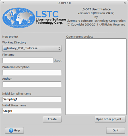
- Create a Working Directory in the desired location e.g. history_MSE_multicase.
- Extract all the files for the example (Windows / Linux) into the working directory.
- Load the history_mse.lsopt file located in the history_MSE_multicase by selecting from the Open other project. This is done in order to reduce repetative steps from the previous example.
- The main GUI window of LS-OPT opens.
Home Screen Process Flowchart
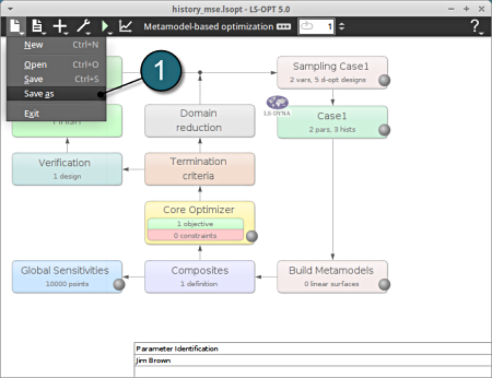
- Select the Save as option from the taskbar. Save the file as history_mse_multicase.lsopt.
Home Screen Process Flowchart
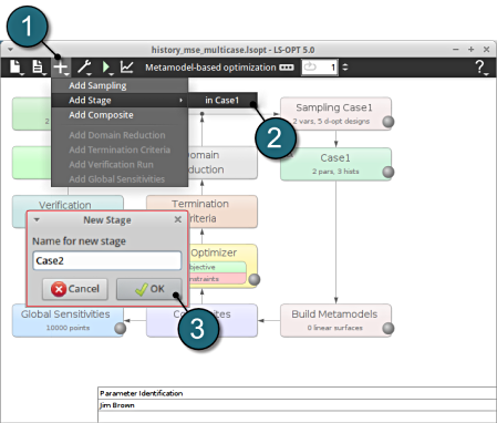
- To add a new Stage select the Add (denoted as +) at the task bar of the GUI.
- Select the Add Stage > in Case1 option. Another possibility to add a similar stage is to use the Clone option when right-clicking an already definied stage. This creates a new stage with the same definitions than the original stage, response and history names are replaced for uniqueness.
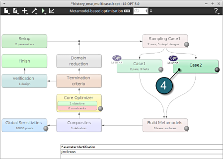
- Select a suitable name for the new stage e.g. Case2 and press OK . The main LS-OPT GUI includes a new Stage Case2 (see image below).
- Select the Case2 box.
A window Stage Case2 shall open.
Define Input File Name and Command
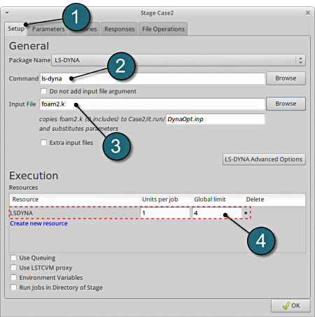
- Select the Setup tab.
- For Command specify the LS-DYNA executable ls-dyna (This name can be different on your computer). On Windows, the command has to be specified using the absolute path.
- For Input File browse for the parameterized file foam2.k. Parameters in LS-DYNA input files can be definied using *PARAMETER or the LS-OPT parameter format <<>>, see Parameters tab.
- For efficient usage of the computing power of the machine, choice on handling the number of concurrent jobs can be made suitably in this section. (E.g., if the machine has 4CPUs, and to run each job on a single CPU : Units per job = 1, Global limit = 4).
The parameters located in the selected Input File can be visualized in the adjoining tab Parameters.
Design Parameters.
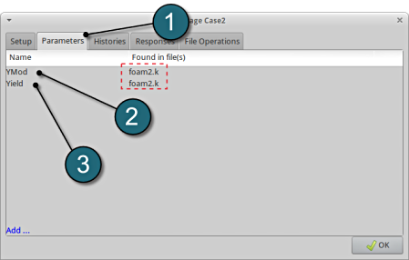
- Select the Parameters tab.
- The first design parameter of the objective function located in the input file foam2.k is displayed ( Young's modulus E (YMod) of the foam material ).
- The second design parameter of the objective function located in the input file foam2.k is displayed ( Yield stress Y (Yield) of the foam material ).
Extract First History
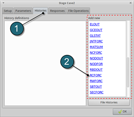
- Select the Histories tab.
- Select the suitable History definition from the available LS-DYNA output interfaces available from the list under Add new, in this case select the option RCFORC.
A separate window emerges named, New history. This enables the user to define the history in suitable steps.
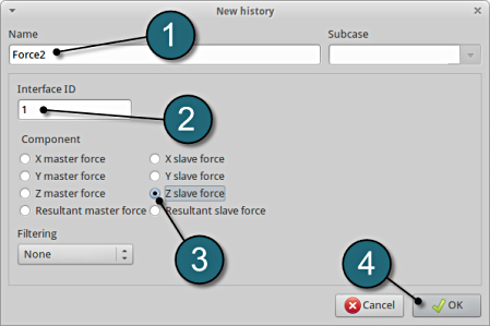
Define z-slave-force on interface 1
- Enter the label Force2 as History name.
- Enter 1 for the Interface ID.
- Select Z slave force for the Component.
- Select OK to proceed.
- This will extract the Z-slave history Force from the binary LS-DYNA output database RCFORC.
- The New history tab closes and returns to the main page of the HIstories tab in the Stage Case2 window.
Add Second History
For additional history definitions from the available LS-DYNA output interfaces available from the list under Add new, select the option NODOUT.
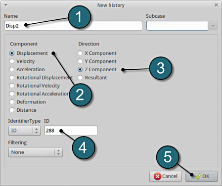
Define z-displacement of node 288
- Enter the label Disp2 as History name.
- For Component select Displacement.
- For Direction select Z Component.
- Type in the node ID: 288.
- Select OK to add the history definition.
This will extract the Z-component of the displacement at node ID 288 from the binary LS-DYNA output database NODOUT.
Add Third History
For additional history definitions, select the option Crossplot available from the list under Add new.
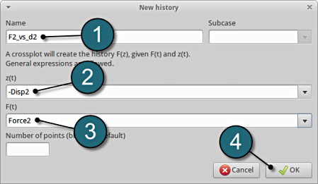
Define crossplot for -Disp2 and Force2
- Type in F2_vs_d2 as History Name.
- For z(t) type in -Disp2 (negative Disp2).
- For F(t) type in Force2.
- Select OK to add the history definition.
This will generate the force vs. displacement curve.
Add File History
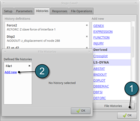
- Select the option File Histories.
A separate window emerges named, File Histories.
Define a history through a text file
- To define an additional file history for use as target curve select the option Add new.
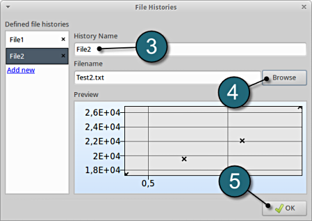
- Type in File2 as History Name.
- Push the Browse button to find the file Test2.txt from your working directory (see below).
- Select OK to add the file history.
  0.36168 17393
  0.72562 19559
  1.0903  22098
  1.4538  26833
*Test2.txt file includes data for 'Displacement' vs. 'Force Resultant'.
History Review
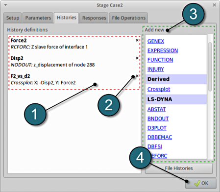
- The defined histories can be reviewed in the tab of the Histories under the History definition. Necessary changes can be made by selecting the choice.
- To delete a History definition click on the cross button (denoted as X).
- Additional histories can be added from the choice available under the Add new list as earlier.
- Select the OK button to proceed.
Home Screen Process Flowchart
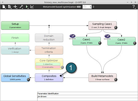
- Select the Composites box.
A window Composites shall open.
Composite Definition
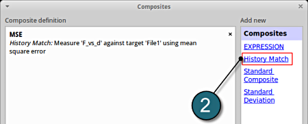
- Select the option History Match for the type of composite under the list for Add new.
A separate window named as History matching composites shall open.
Define Composite
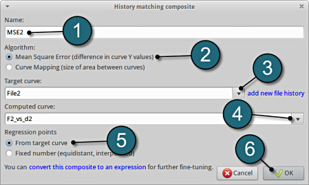
- Enter the Name for composite as MSE2.
- Select the option Mean Square Error for the options from Algorithm.
- For Target curve select FILE2.
- For Computed curve select F2_vs_d2.
- The selection of Regression points is kept at From target curve (default).
- Select OK to add the composite definition.
- The main difference between the above mentioned algorithm has been explained in details on this page.
Composites Review
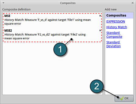
- The defined composites can be reviewed in the main page of the Composites under the Composite definition. Necessary changes can be made by selecting the choice.
- Select OK to continue.
Home Screen Process Flowchart
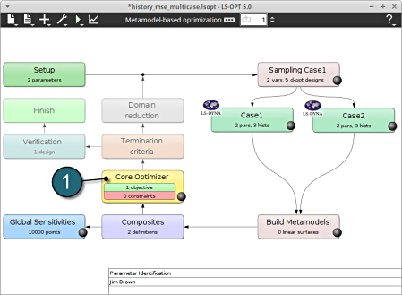
- Select the Optimization box.
A window Algorithms shall open.
Add Objective
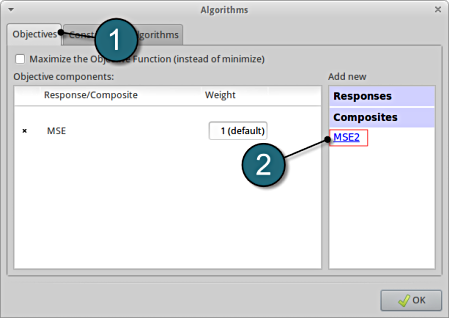
- Select the Objectives tab.
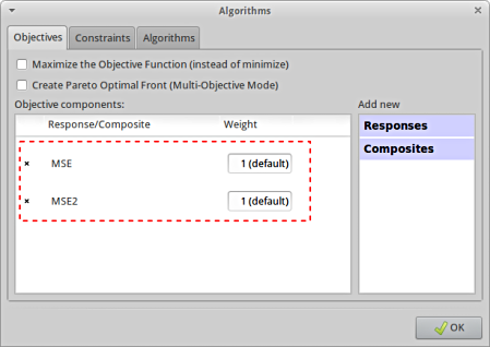
- Add MSE2 as an addition objective.
Define Objective
For Weight leave the default 1. If you have several objective functions, you may assign weight to each one according to their importance.
LS-OPT will minimize the weighted sum of the componentes, in this case
MSE + MSE2
Optimization Algorithm.
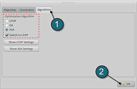
- Select the Algorithms tab. Here, the algorithm used for the optimization on the metamodel can be selected.
- Make sure that the radio button for Adaptive Simulated Annealing (ASA) is selected and Switch to LFOP is checked. These are the default settings.
- Select the OK button to proceed.
Home Screen Process Flowchart
-
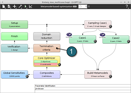
Select the Termination criteria icon.
A window Termination criteria shall open.
Define the Termination criteria
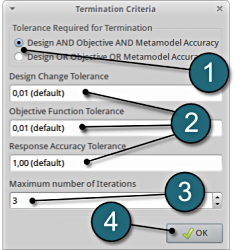
- Retail the (default) selection of the radio button on Design AND Objective AND Metamodel Accuracy for the choice of Tolerance Required for Termination.
- Several Tolerance parameters (Design, Objective, Response) are retained to their default values.
- Change the Maximum number of Iterations to 3.
- Push the OK button to proceed.
Run LS-Opt.
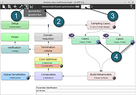
- Select the Run button from the Control Bar.
- Push Normal Run for execution.
- The user can get information on the status of the current iteration during execution.
- At every stage the user has an option to view the progress of the program execution by selecting the LED on the Stage tabs. either Case1 or Case2 tab.
As seperate window Progress opens up.
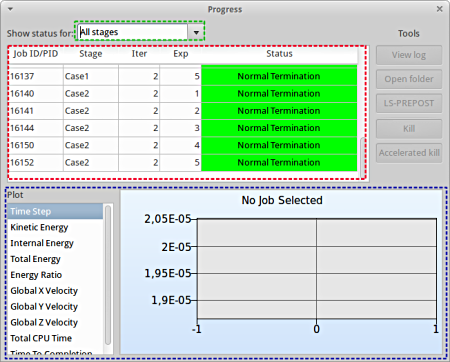
Progress
- Change the status of Show status for option to All stages for visualization .
- The progress bar gives information on the status and several other details of the optimization progress.
- Underneath the status, the user has the option to view various plots of the computed values during execution vs the simulation time.
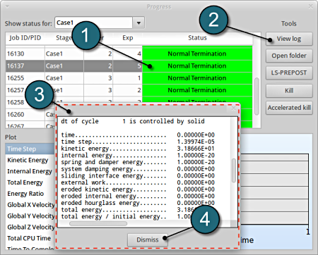
View Log
- Select the simulation point for which the log file is desired.
- Click on the View log button.
- A new window opens containing the solver output, in this case the LS-DYNA output.
- Select the Dismiss button to close the window and proceed.
-
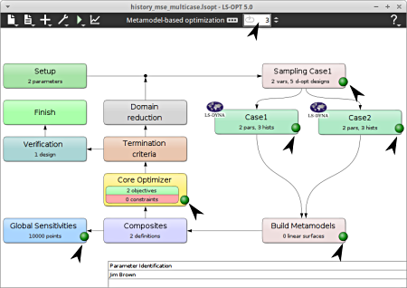
To view the status of the program during execution, observe the grey LED's at every stage of the process flow. Succesful completion of every stage is marked by turning respective LED green.
-
The iterations count at the taskbar can be altered to observe the activities at various iterations.
After completion of the program execution the user can view the results.
Home Screen Process Flowchart
- The results can be viewed by selecting the view button on the task bar. A seperate window of LS-OPT Viewer opens up.
LS-OPT Viewer
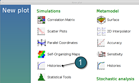
- Select under Simulations the item Histories.
Plot Setup
Setup the top panel for Case1
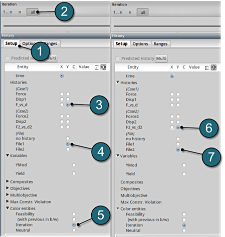
- Select the Setup tab.
- Select all for the iterations setup.
- Plot coordinate selections for Y-axis is made as F_vs_d.
- Select File1 to plot the test data together with the simulation results.
- Choose Iterations for the Color entities.
- To set up an additional plot select the split option form the task bar (encirled in figure below).
Setup the top panel for Case2
- Plot co-ordinate selections for Y-axis made as F2_vs_d2.
- Select File2 to plot the test data together with the simulation results.
Plot
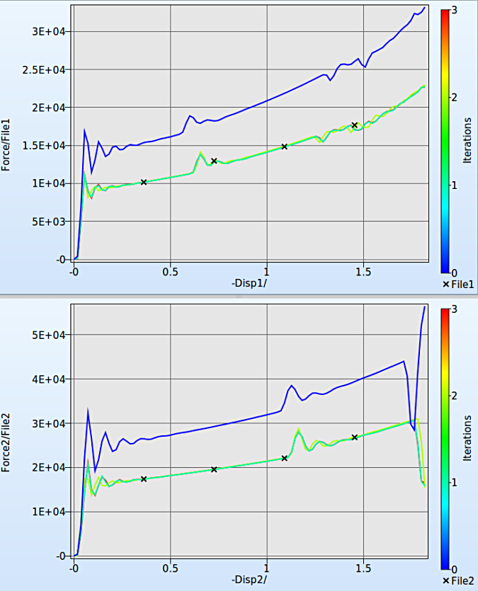
- The two 2-D plots clearly shows the optimal simulation curves at different iterations for the crossplot of Force vs -Disp1 and Force2 vs -Disp2 (shown below).
- The crosses (denoted as x) mark out the "experimental" result stored in FILE1 and FILE2 in order to compare themself with the simulation result. We can see, they are well-matched at the subsiquient iterations.
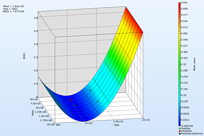
We can plot the several surface plots of the metamodel we've built. For example, we want to see a surface plot of the objective function MSE or MSE2 with respect to the variables YMod and Yield, do it as following:
New Plot
- To view a new plot select the plot button on the task bar. A seperate window of LS-OPT Viewer opens up.
LS-OPT Viewer
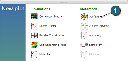
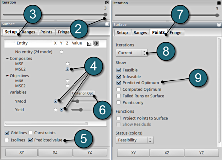
- Select under Metamodel the item Surface.
- Slide to the last iteration.
- Select the Setup tab.
- Set MSE2 as the z-coordinate, the variables YMod and Yield as the x-coordinate and y-coordinate, respectively.
- Choose Predicted value. A purple cross will appear somewhere on the surface. You can move it by changing the values of the variables YMod and Yield using the repective sliders. The predicted value for the selected parameter combination is displayed.
- Click Center on Opt. to locate the cross at the optimal point.
- Select the Points tab.
- Make the selection for Iterations at Current.
- Pick Predicted Optimum and Computed Optimum.
- In the similar way, we can visulaize the metamodel surface for the MSE with respect to the input parameters.
Note that the surface plot for MSE2 shows a quadratic surface, although we used linear polynomials. The reason is that Mean Square Error estimate is defined as a composite expression that is calculated using the metamodels of the components, and the expression is of quadratic order.
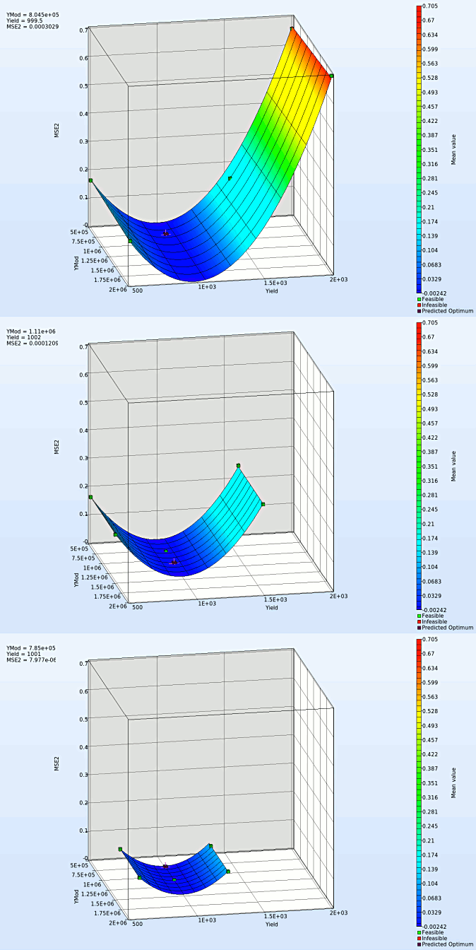
- We rotate the plot with the mouse by pressing Ctrl at the meantime. We can change the surface plot for each iteration (at step 2.) and visualize the effect of domain reduction (as shown below).
Fig. Effect of domain reduction on optimization process
What is the approximation error of the result?
The approximation error indicators (predict the metamodel accuracy of the results) can be visualized in the LS-OPT Viewer.
New Plot
- To view a new plot select the plot button on the task bar. A seperate window of LS-OPT Viewer opens up.
LS-OPT Viewer
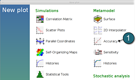
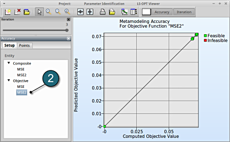
- Select under Metamodel the item Accuracy.
- From Entity select the Objective MSE2.
→ Good approximation: low distance between black line and green points.
→Similar observations can be made by selecting the other objective MSE.
Optimization History
- Alternatively the accuracy of the optimal MSE values at various iterations can be studied under a Optimization History plot.
New Plot
- To view a new plot select the plot button on the task bar. A seperate window of LS-OPT Viewer opens up.
LS-OPT Viewer
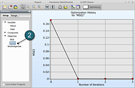
- Select under Optimization the item History.
- From Setup tab, select the Objective MSE2..
→ Good approximation of optima: The computed values (red points) almost coincide with the predicted values (black line).
→Similar observations can be made by selecting the other objective MSE.
New Plot
- To view a new plot select the plot button on the task bar. A seperate window of LS-OPT Viewer opens up.
LS-OPT Viewer
- Choose History under the category Optimization.
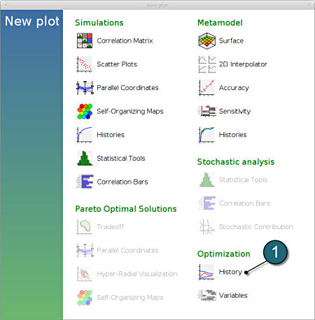
- We can choose from the left side the entities we want to observe.
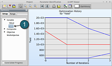
1. Select Variable → Yield
Fig. 1(a) shows:
- The optimization history of the variable Yield.
- The development of the variable value of the optimum (red line)
- How the range of Yield (set from 2000 to 500 at the beginning) decreases after every iteration (blue lines).
- This variable is important (see Sensitivities) to minimize the objective, and seems to be converged.
Fig. 1(a)
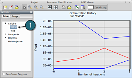
1. Select Variable → YMod
Fig. 1(b) shows:
- The optimization history of the variable YMod.
- The development of the optimal variable value (red line)
- How the range of YMod (set to 2000000 to 500000 at the beginning) decreases after every iteration (blue lines).
- This variable is rather insignificant (see Sensitivities) and therefor differs between the iteration without affecting the objective.
Fig. 1(b)
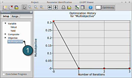
1. Select Objective → Multiobjective
Fig. 1(c) shows:
- The predicted result (black line) of the optimal objective Multiobjective (MSE and MSE2) for every iteration.
- The computed result (red points) of the optimal objective Multiobjective for every iteration.
- The convergence trend of the Multiobjective.
Fig. 1(c)
New Plot
- To view a new plot select the plot button on the task bar. A seperate window of LS-OPT Viewer opens up.
LS-OPT Viewer
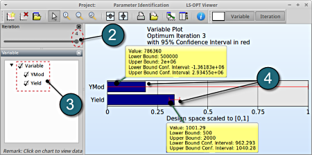
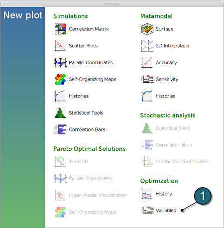
- Choose Variables under the category Optimization.
- Drag the Iteration to 4.
- The Variable selection for YMod and Yield are already selected by default.
- The user can view the Confidence Intervals and other bounds by double clicking on the respective bar plots.
-
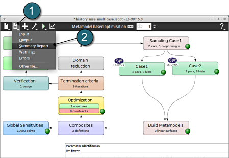
Alternatively the Confidence Intervals can be found in the lsopt_report file. The user can access the file by the following steps:
LS-OPT GUI
- Select the Files menu located in the control bar.
- Select the option Summary Report from the list.
A seperape file shall open, search for the term Confidence Interval at Iteration 4 (see file below).
The file lsopt_report is located in the working directory and can also be opened using any text editor.
=========================================================
                 C O N F I D E N C E   I N T E R V A L S

                              ITERATION 4
===========================================================

------------------------------------------------------------
 95% Confidence intervals for individual optimal parameters
------------------------------------------------------------
Name                  Value              Confidence
                                          Interval
                                      Lower      Upper
------------------------------------------------------------
YMod             786359.819         1361832.8  2934552.47
Yield            1001.28693        962.293152  1040.2807
------------------------------------------------------------
Which variable appears to be the most important?
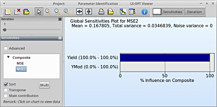
The significance of a variable for a response can be illustrated with ANOVA (analysis of variance) or GSA/Sobol (global sensitivity analysis). In this case, only GSA is available, since ANOVA is only calculated for responses, not for composites.
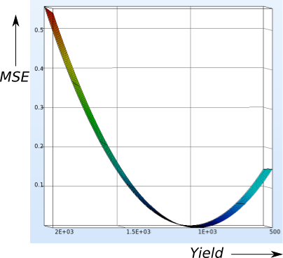
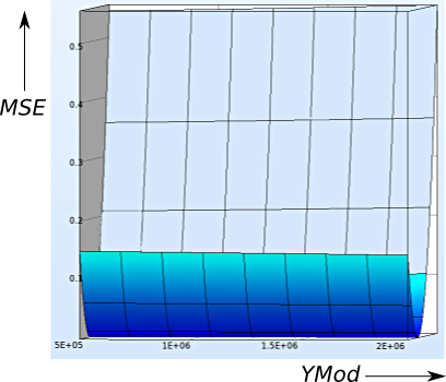
- The same inference can be drawn from the surface plot which clearly depicts that the variable YMod (fig. right side) makes neglible change in the value of MSE.
- Whereas a similar plot with the variable Yield proves the sensitivity on the objective MSE.
- For problems with more parameters, only sections of the metamodels can be displayed, hence sensitivites are not always that obvious.
New Plot
- To view a new plot select the plot button on the task bar. A seperate window of LS-OPT Viewer opens up.
LS-OPT Viewer
GSA/Sobol
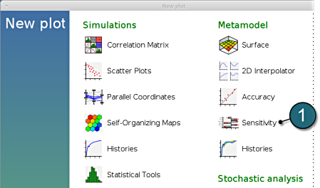
- Restart the LS-OPT Viewer and select under Metamodel the item Sensitivity
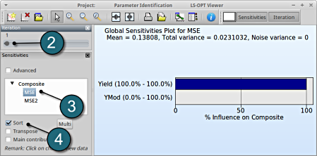
- We can slide to observe the sensitivity of results at each iteration. In this case for Iteration 1.
- Select MSE from the Composite.
- Select Sort for the variables.
→ For the composite MSE the variable Yield is more important, while the variable YMod is rather insignificant.
→ Similar observation can be made for the other composite MSE2 upon selection.

