Solution with LS-OPTui
https://www.lsoptsupport.com/examples-4.0/subpages/metaforming/solution-with-ls-optui
https://www.lsoptsupport.com/@@site-logo/LS-Opt-Support-Logo480x80.png
Solution with LS-OPTui
Monto Carlo Analysis Task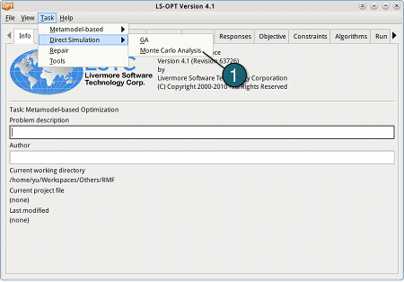
- From the main menu bar select Task → Direct Simulation → Monto Carlo Analysis.
Define the solver
- Select the Solvers panel.
- For Solver Package Name choose LS-DYNA.
- For Command specify the LS-DYNA executable ls971_R4_2 (This name can be different on your computer).
- For Input File browse the file metal.k.
- For Name of Analysis Case enter SOLVER_1.
- Push the Add button.
Statistical Distribution
- Select the Distribution panel.
- Choose Normal Type.
- For Mean enter 200.
- For Standard Dev enter 20.
- Type in a Distribution Name, e.g. Y.
- Push the Add button.
- Choose Uniform Type.
- For Lower enter 0.6.
- For Upper enter 1.4.
- Type in a Distribution Name, e.g. U_FS.
- Push the Add button.
- Choose Uniform Type.
- For Lower enter 0.
- For Upper enter 50.
- Type in a Distribution Name, e.g. P_OFF.
- Push the Add button.
Change Variable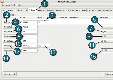
- Select the Variables panel. The variables are already defined in the input file metal.k using *PARAMETER (see below) and therefore cannot be deleted.
- For Type of NAdapt switch the menu to Constant.
Change the (start) value of NAdapt to 2.
- For Type of YIELD switch the menu to Noise Var.
- Choose Y as the Distribution of the variable YIELD.
- For Type of FS1 switch the menu to Noise Var.
- Choose U_FS as the Distribution of the variable FS1.
- For Type of FS2 switch the menu to Noise Var.
- Choose U_FS as the Distribution of the variable FS2.
- For Type of FS3 switch the menu to Noise Var.
- Choose U_FS as the Distribution of the variable FS3.
- For Type of PWAVEL switch the menu to Constant.
- Change the (start) value of PWAVEL to 50.
- For Type of POFF switch the menu to Noise Var.
- Choose P_OFF as the Distribution of the variable POFF.
Sampling Panel
- Select the Sampling Panel.
- For POINT SELECTION choose Latin Hypercube.
- For Number of Simulation Points per Case enter 25.
Define the Responses
Define the maximum percent thinkness reduction
- Select the Responses panel.
- From the possible response types select: D3PLOT.
- For Parts to be included choose All Parts.
- For Result Type select Misc.
- For Component select %_thickness_reduction.
- And select the Maximum Value.
- And the maximum value should be taken from time 0 to the current time.
- For Response Name enter prc_thick_red_max.
- Push the Add button.
Define the FLD
- From the possible response types select: FLD.
- For Parts to be included choose List of Parts.
- In the List of Parts enter 1.
- Push the (Add) > button.
Repeat the previous steps and create this list of parts:
| List of Parts: |
|---|
1 |
| 2 |
| 3 |
- For Sampling locatin select Center surface.
- For Load curve ID enter 90.
- For Response Name enter PLD.
- Push the Add button.
Define the minimum shell thickness
- From the possible response types select: D3PLOT.
- For Parts to be included choose List of Parts.
- In the List of Parts enter 1.
- For Result Type select Misc.
- For Component select shell_thickness.
- And select the Minimum Value.
- And the minimum value should be taken from time 0 to the current time.
- For Response Name enter thick_min.
- Push the Add button.
Define the objective response
- Select the Objective panel.
- From Response select prc_thick_red_max as the objective.
- For Weight leave the default 1. If you have several objective functions, you may assign weight to each one according to their importance.
Define the constraints
- Select the Constraints panel.
- Choose the Response per_thick_red_max as constraint.
- For Lower Bound accept the default -inf.
- For Upper Bound enter 34.
Run panel
- Select the Run panel.
- Push the Run button. (Save the project as com.metal_MC)
$$$$$$$$$$$$$$$$$$$$$$$$$$$$$$$$$$$$$$$$$$$$$$$$$$$$$$$
Command file "com.metal_MC"
$$$$$$$$$$$$$$$$$$$$$$$$$$$$$$$$$$$$$$$$$$$$$$$$$$$$$$$
$ Generated using LS-OPT Version 4.1
$
"Metalforming Analysis Example Problem"
$
Author "LS-OPT Class"
$ Created on Tue Apr 26 16:29:24 2011
solvers 1
responses 3
$
$ NO HISTORIES ARE DEFINED
$
$
$ PROBABILISTIC DISTRIBUTIONS
$
distribution 3
 distribution 'Y' NORMAL  200  20
 distribution 'U_FS' UNIFORM  0.6  1.4
 distribution 'P_OFF' UNIFORM  0  50
$
$ DESIGN VARIABLES
$
variables 5
 Noise variable 'YIELD' distribution 'Y'
 Noise variable 'FS1' distribution 'U_FS'
 Noise variable 'POFF' distribution 'P_OFF'
 Noise variable 'FS2' distribution 'U_FS'
 Noise variable 'FS3' distribution 'U_FS'
$
$ CONSTANTS
$
constants 2
 Constant 'PWAVEL' 50
 Constant 'NAdapt' 2

$$$$$$$$$$$$$$$$$$$$$$$$$$$$$$$$
$      SOLVER "SOLVER_1"
$$$$$$$$$$$$$$$$$$$$$$$$$$$$$$$$
$
$ DEFINITION OF SOLVER "SOLVER_1"
$
 solver dyna960 'SOLVER_1'
  solver command "ls971_R4_2"
  solver input file "metal.k"
  solver check output on
  solver compress d3plot off
$ ------ Pre-processor --------
$   NO PREPROCESSOR SPECIFIED
$ ------ Post-processor --------
$   NO POSTPROCESSOR SPECIFIED
$ ------ Metamodeling ---------
  solver experiment design lhd_generalized
  solver number experiments 25
$ ------ Job information ------
  solver concurrent jobs 1
$
$ RESPONSES FOR SOLVER "SOLVER_1"
$
 response 'prc_thick_red_max' 1 0 "D3PlotResponse
  -res_type misc  -cmp %_thickness_reduction -select MAX -start_time 0.0000"
 response 'FLD' 1 0 "DynaFLDg CENTER 1 2 3 90"
 response 'thick_min' 1 0 "D3PlotResponse -pids 1
  -res_type misc  -cmp shell_thickness -select MIN -start_time 0.0000"

$
$ OBJECTIVE FUNCTIONS
$
 objectives 1
 objective 'prc_thick_red_max' 1
$
$ CONSTRAINT DEFINITIONS
$
 constraints 1
 constraint 'prc_thick_red_max'
  upper bound constraint 'prc_thick_red_max' 34
$
$ JOB INFO
$
analyze monte carlo
STOP