Accuracy
New Plot
- To view a new plot select the plot botton on the task bar. A seperate window of LS-OPT Viewer opens up.
LS-OPT Viewer
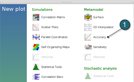
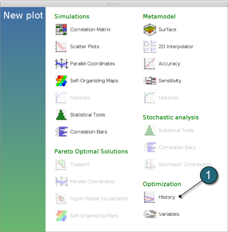
- Select under Metamodel the item Accuracy.
RMS Error and R2 Indicator
- From the left side of the window select Responses → HIC.
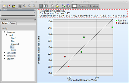
- RMS Error, SPRESS and R2 (R-sq) can be found above the plot.
- We can slide to observe the accuary of results at each iteration. In this case for Iteration 1.
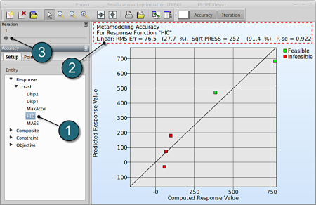
- At the last iteration (Iteration 8) we obtain a result with RMS Error = 5.39 (4.17%) and R2 = 0.801.
- A small RMS error and a coefficient of determination (R2) ~1 indicates good fit (see table below).
- A relatively low SPRESS (=13.5%) is observed which indicates a good prediction of the metamodel.
| RMS Error | R2 Indicator | |
| Small | ~1 | High variable detection: low noise, good fit. |
| Small | ~0 | Low noise/good fit, small gradient. |
| Large | ~1 | High variable detection with noise. |
| Large | ~0 | Lack of fit, perhaps accompanied by noise. Must shrink the move limits. |
We can find the development of RMS Error and R2 in History under Optimization.
New Plot
- To view a new plot select the plot botton on the task bar. A seperate window of LS-OPT Viewer opens up.
LS-OPT Viewer
- Choose History under the category Optimization.
- Select from the left of the window Response → HIC
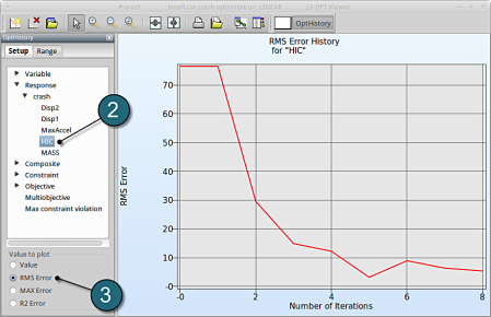
- Select RMS Error. We see that the RMS error is large at the 1st iteration and progressivly reduces till the 5th iteration.
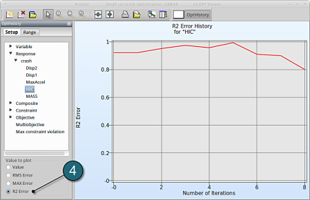
- Select R2 Error. The R2 error reaches its maximum near 1 at the 5th iteration, and then starts decreasing again.
