Convergence
Home Screen Process Flowchart
- The results can be viewed by selecting the view button on the task bar. A seperate window of LS-OPT Viewer opens up.
LS-OPT Viewer
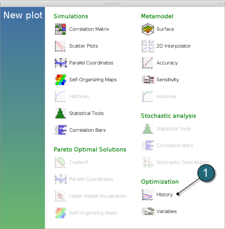
- Choose History under the category Optimization.
- We can choose from the left side the entities we want to observe.
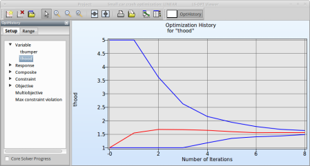
Select Variables → thood
Fig. 1(a) shows:
- The optimization history of the variable thood.
- The development of the variable value of the optimum (red line)
- How the range of thood (set from 1 to 5 at the beginning) decreases after every iteration (blue lines).
- This variable is important (see Sensitivities) to reach the bounds of the constraint and minimize the objective and seems to be converged.
Fig. 1(a)
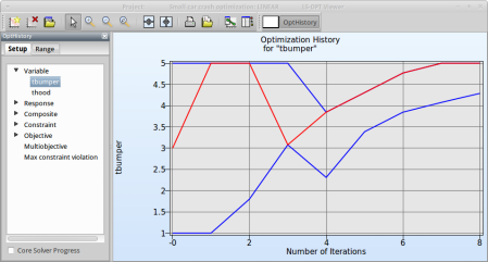
Select Variable → tbumper
Fig. 1(b) shows:
- The optimization history of the variable tbumper.
- The development of the optimal variable value (red line)
- How the range of tbumper (set to 1...5 at the beginning) decreases after every iteration (blue lines).
- This variable is rather insignificant (see Sensitivities) and therefor differs between the iteration without affecting the objective.
Fig. 1(b)
As you can see in the figure the value of thood doesn't change a lot between iteration 7 and 8. The tolerance for termination of 1% is reached and this will make LS-OPT stop the optimization process after 8 iterations although 10 iterations were specified in the Run panel.
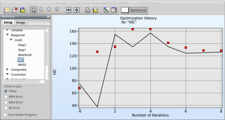
Select Response → crash → HIC
Fig. 2(a) shows:
- The predicted result (black line) of the optimal HIC response for every iteration.
- The computed result (red points) of the HIC response for every iteration.
- The convergence trend of the HIC response.
From the starting value to the optimum of the first iteration, the objectives increases to satisfy the constraint that is violated for the starting design, see Fig. 2(b).
Fig. 2(a)
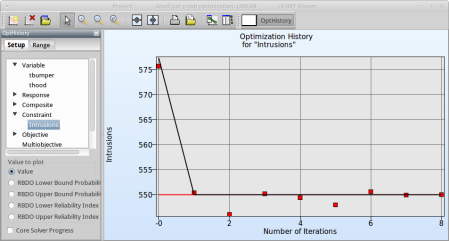
Select Constraint → Intrusions
Fig. 2(b) shows:
- The predicted result (black line) of the optimal Intrusion constraint for every iteration.
- The computed result (red points) of the Intrusion constraint for every iteration.
- The constraint upper bound is reached (red line).
Fig. 2(b)

