Results
Home Screen Process Flowchart
- The results can be viewed by selecting the view button on the task bar. A seperate window of LS-OPT Viewer opens up.
LS-OPT Viewer
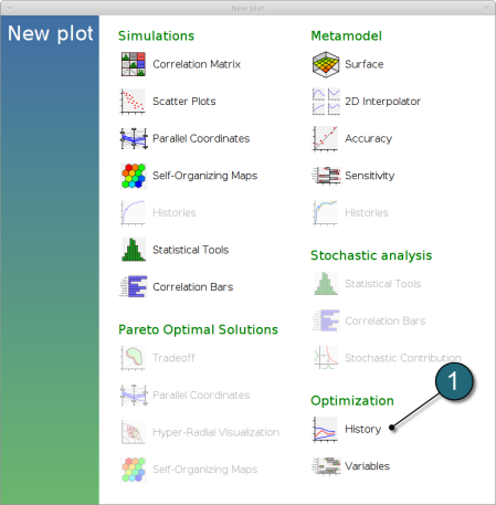
- Choose History under the category Optimization.
- We can choose from the left side the entities we want to observe.
Select Variables → thood
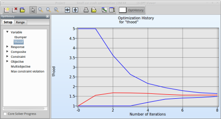
Fig. 1(a) shows:
- The optimization history of the variable thood.
- The development of the variable value of the optimum (red line)
- How the range of thood (set from 1 to 5 at the beginning) decreases after every iteration (blue lines).
- This variable is important (see Sensitivities) to reach the bounds of the constraint and minimize the objective and seems to be converged.
Fig. 1(a)
Select Variable → tbumper
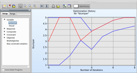
Fig. 1(b) shows:
- The optimization history of the variable tbumper.
- The development of the optimal variable value (red line)
- How the range of tbumper (set to 1...5 at the beginning) decreases after every iteration (blue lines).
- This variable is rather insignificant (see Sensitivities) and therefor differs between the iteration without affecting the objective.
Fig. 1(b)
As you can see in the figure the value of thood doesn't change a lot between iteration 7 and 8. The tolerance for termination of 1% is reached and this will make LS-OPT stop the optimization process after 8 iterations although 10 iterations were specified in the Run panel.
Select Response → crash → HIC
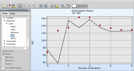
Fig. 2(a) shows:
- The predicted result (black line) of the optimal HIC response for every iteration.
- The computed result (red points) of the HIC response for every iteration.
- The convergence trend of the HIC response.
From the starting value to the optimum of the first iteration, the objectives increases to satisfy the constraint that is violated for the starting design, see Fig. 2(b).
Fig. 2(a)
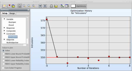
Select Constraint → Intrusions
Fig. 2(b) shows:
- The predicted result (black line) of the optimal Intrusion constraint for every iteration.
- The computed result (red points) of the Intrusion constraint for every iteration.
- The constraint upper bound is reached (red line).
Fig. 2(b)
New Plot
- To view a new plot select the plot botton on the task bar. A seperate window of LS-OPT Viewer opens up.
LS-OPT Viewer
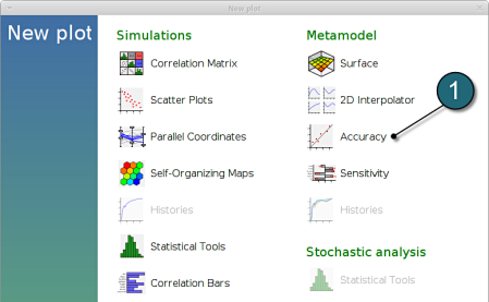
- Select under Metamodel the item Accuracy.
RMS Error and R2 Indicator
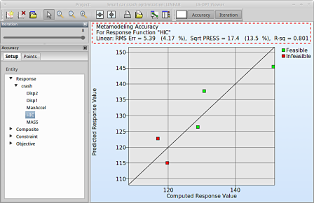
- From the left side of the window select Responses → HIC.
- RMS Error, SPRESS and R2 (R-sq) can be found above the plot.
- We can slide to observe the accuary of results at each iteration. In this case for Iteration 1.
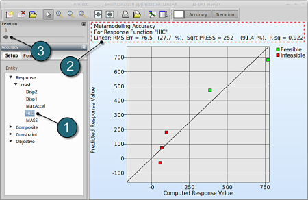
- At the last iteration (Iteration 8) we obtain a result with RMS Error = 5.39 (4.17%) and R2 = 0.801.
- A small RMS error and a coefficient of determination (R2) ~1 indicates good fit (see table below).
- A relatively low SPRESS (=13.5%) is observed which indicates a good prediction of the metamodel.
| RMS Error | R2 Indicator | |
| Small | ~1 | High variable detection: low noise, good fit. |
| Small | ~0 | Low noise/good fit, small gradient. |
| Large | ~1 | High variable detection with noise. |
| Large | ~0 | Lack of fit, perhaps accompanied by noise. Must shrink the move limits. |
We can find the development of RMS Error and R2 in History under Optimization.
New Plot
- To view a new plot select the plot botton on the task bar. A seperate window of LS-OPT Viewer opens up.
LS-OPT Viewer
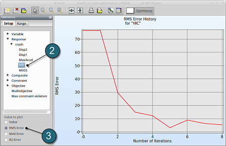
- Choose History under the category Optimization.
- Select from the left of the window Response → HIC
- Select RMS Error. We see that the RMS error is large at the 1st iteration and progressivly reduces till the 5th iteration.
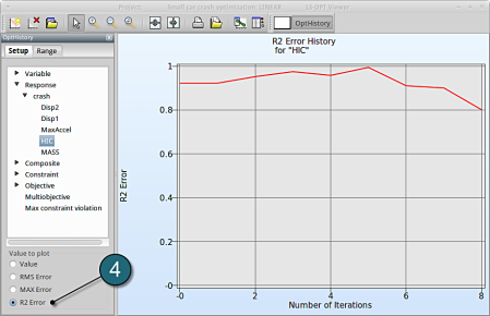
- Select R2 Error. The R2 error reaches its maximum near 1 at the 5th iteration, and then starts decreasing again.
We can plot the response surface of the metamodel we've built. For example, we want to see the response surface of HIC with respect to the variables thood and tbumper, do it as following:
New Plot
- To view a new plot select the plot botton on the task bar. A seperate window of LS-OPT Viewer opens up.
LS-OPT Viewer
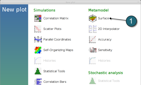
- Select under Metamodel the item Surface.
- Slide to the last iteration.
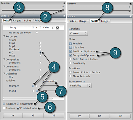
- Select the Setup tab.
- Set the response HIC as the z-coordinate, the variables tbumper and thood as the x-coordinate and y-coordinate, respectively.
- Pick Constraints to visualize feasible and infeasible regions on the metamodel, respectively. The feasible region is drawn in green while the infeasible region is drawn in red.
- Choose Predicted value. A purple cross will appear somewhere on the surface. You can move it by changing the values of the variables tbumper and thood. The predicted value for the selected parameter combination is displayed.
- Click Center on Opt. to locate the cross at the optimal point.
- Select the Points tab.
- Pick Predicted Optimum and Computed Optimum.
- We rotate the plot with the mouse by pressing Ctrl at the meantime. The purple cube shows the predicted optimum value, while the red cube above denotes the computed optimum value, which is computed directly through the simulation model. Red indicates that the point is infeasible.
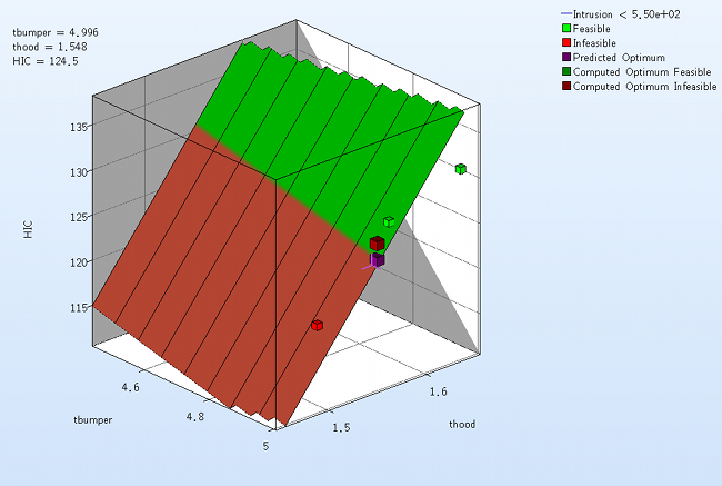
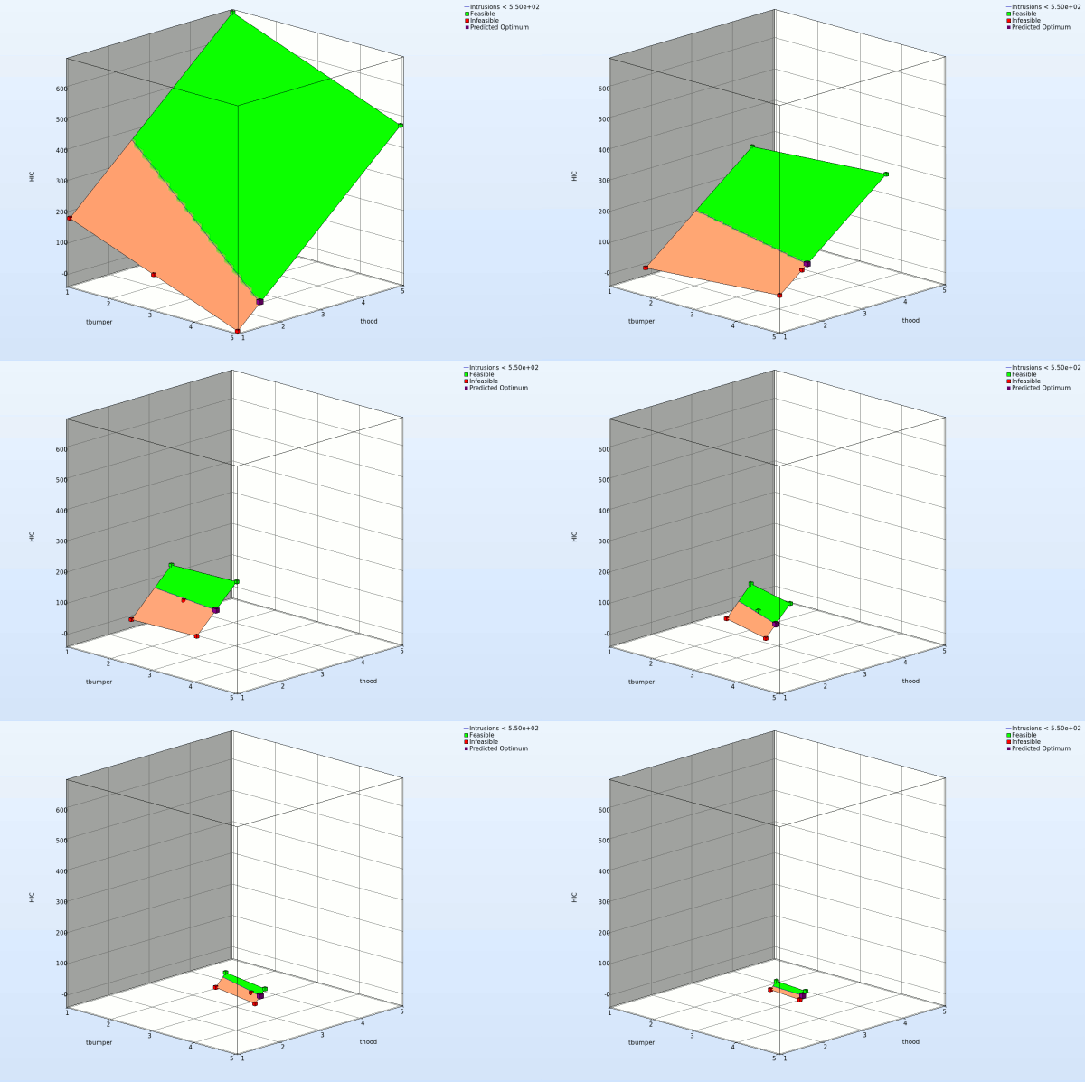
Fig. Effect of domain reduction on optimization process
Which variable appears to be the most important?
The significance of a variable for a response can be illustrated with ANOVA (analysis of variance) or GSA/Sobol (global sensitivity analysis), e.g for the response HIC you may find:
New Plot
- To view a new plot select the plot botton on the task bar. A seperate window of LS-OPT Viewer opens up.
LS-OPT Viewer
ANOVA
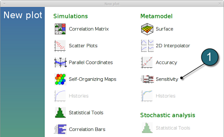
- Restart the LS-OPT Viewer and select under Metamodel the item Sensitivity
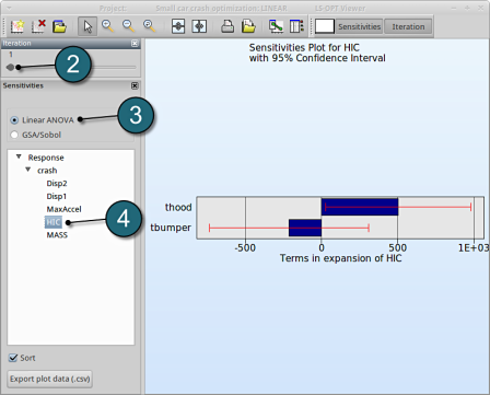
- We can slide to observe the sensitivity of results at each iteration. In this case for Iteration 1.
- Select Linear ANOVA in the new window.
- From Response select HIC.
→ For the response HIC the variable thood is more important, while the variable tbumper is rather insignificant.
GSA/Sobol
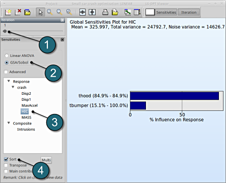
- The sensitivity analysis is done at Iteration 1, because of the domain reduction.
- Select GSA/Sobol.
- From Response select HIC.
- Sort the variables according to their significance for HIC.
→ We come to the same conclusion by using GSA. The influence of thood on HIC is 84.9%, larger than that of tbumper with 15.1%.

