Surface

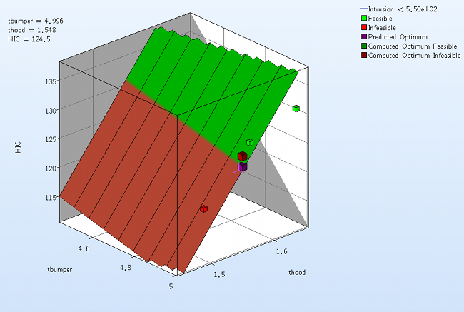
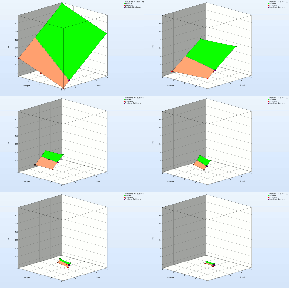
We can plot the response surface of the metamodel we've built. For example, we want to see the response surface of HIC with respect to the variables thood and tbumper, do it as following:

New Plot

• To view a new plot select the plot botton on the task bar. A seperate window of LS-OPT Viewer opens up.

LS-OPT Viewer

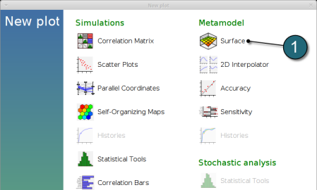
1. Select under Metamodel the item Surface.
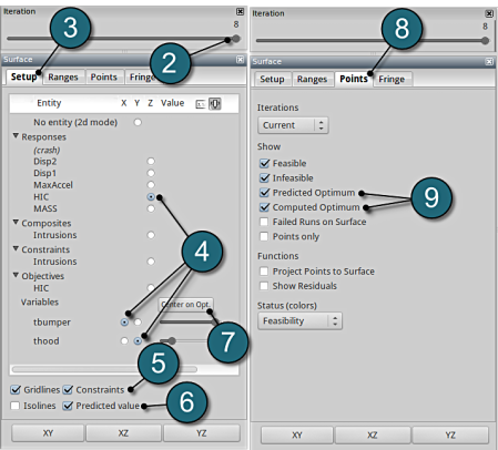
2. Slide to the last iteration.
3. Select the Setup tab.
4. Set the response HIC as the z-coordinate, the variables tbumper and thood as the x-coordinate and y-coordinate, respectively.
5. Pick Constraints to visualize feasible and infeasible regions on the metamodel, respectively. The feasible region is drawn in green while the infeasible region is drawn in red.
6. Choose Predicted value. A purple cross will appear somewhere on the surface. You can move it by changing the values of the variables tbumper and thood. The predicted value for the selected parameter combination is displayed.
   
7. Click Center on Opt. to locate the cross at the optimal point.
8. Select the Points tab.
9. Pick Predicted Optimum and Computed Optimum.

• We rotate the plot with the mouse by pressing Ctrl at the meantime. The purple cube shows the predicted optimum value, while the red cube above denotes the computed optimum value, which is computed directly through the simulation model. Red indicates that the point is infeasible.