Computed vs. Predicted
Study the change in each of the variables/responses and the accuracy of the predicted compared to the computed result.
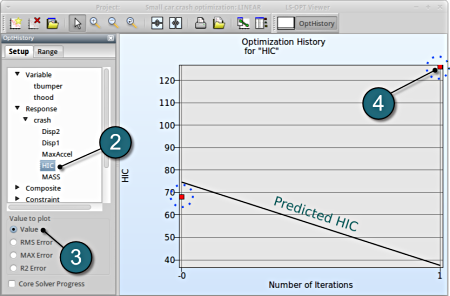
The accuracy of the starting point and the approximate optimum points after the first iteration can be illustrated, e.g. for the response HIC you may find:
New Plot
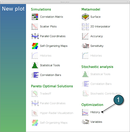
- To view a new plot select the plot botton on the task bar. A seperate window of LS-OPT Viewer opens up.
LS-OPT Viewer
- Select under Optimization the item History.
- From the left side of the window select Responses → HIC.
- For Value to Plot select Value.
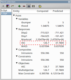
- If you want to see the accurate values, simply click nearby the red points. There appears a table, which states all the computed and predicted data, e.g. computed HIC vs. predicted HIC.
→ You can find out the appropriate values for the predicted (black) and the computed (red points) results. More iterations may lead to a better predictive capability.
→ A quality analysis is expected when the predicted (black line) and the computed (red points) are in close proximity.
(Note the range of the values when assessing the accuracy)
Predicted results compared to the computed result.
The user can select the respective points and compare the predicted values to the computed results for every iteration :
| Start ( 0.Opt ) | First Iteration ( 1.Opt ) | |||||||||||||||
| Predicted | Computed | Predicted | Computed | |||||||||||||
| thood | 1 | 1.549 | ||||||||||||||
| tbumper | 3 | 5 | ||||||||||||||
| MASS | 0.4103 | 0.4103 | 0.657 | 0.6571 | ||||||||||||
| Intrusion | 577.3 | 575.7 | 550 | 550.4 | ||||||||||||
| HIC | 74.64 | 68.02 | 37.78 | 126.7 | ||||||||||||
| Max. Constr. Violation | 27.28 | 25.69 | 9.919e-5 | 0.3957 | ||||||||||||


