Surface
We can plot the response surface of the metamodel we've built. For example, we want to see the effect of the constraint on the optimization solution with respect to the variables thood and tbumper, do it as following:
Home Screen Process Flowchart
- The results can be viewed by selecting the view button on the task bar. A seperate window of LS-OPT Viewer opens up.
LS-OPT Viewer
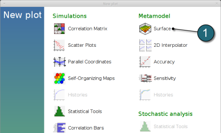
- Select under Metamodel the item Surface.

Constraints
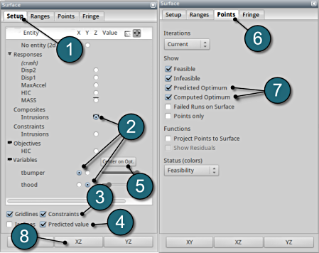
- Select the Setup tab.
- Set the plot coordinates,
- Composites, Intrusions : z-coordinate
- Variables, tbumper : x-coordinate
- Variables, thood : y-coordinate.
- Pick Constraints to visualize feasible and infeasible regions on the metamodel, respectively.
- green : feasible region
- red : infeasible region.
- Choose Predicted value, a cross (+) appears on the surface.
- Click Center on Opt. to locate the cross at the optimal point.
- Select the Points tab.
- Pick Predicted Optimum and Computed Optimum.
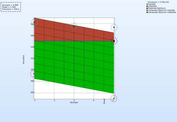
- To view the optimization constraints, we take a 2-D plot of Intrusions vs tbumber (variable).

Plot
- The 2-D plot clearly shows that the points in the red region ( intusions > 550 mm ) form the infeasible solutions, whereas the green points are the feasible solutions.
- The optimum point lies at the periphery of the feasible and infeasible domain. The predicted optimum point values are shown at the top-left corner of the plot.

Objective - HIC Plot
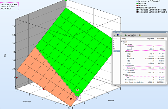
- The primary objective of the optimization is to minmize the HIC.
- Repeat similar steps as the previous plot except for Z-axis select the Objective - HIC.
- Avoid Step. 8, to visulaize in a 3-D plot.
- It is important to note, the optimum is located at the lowest HIC in the feasible region.
- The user has the option to view the various entities by selecting any given point in the plot ( in this case the predicted optimum ). A point selection window opens up.

