Surface
We can plot the several surface plots of the metamodel we've built. For example, we want to see a surface plot of the objective function Residual2 with respect to the variables CB and SIGY, do it as following:
New Plot
- To view a new plot select the plot button on the task bar. A seperate window of LS-OPT Viewer opens up.
LS-OPT Viewer
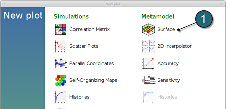
- Select under Metamodel the item Surface.
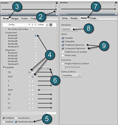
- Slide to the last iteration.
- Select the Setup tab.
- Set Residual2 as the z-coordinate, the variables CB and SIGY as the x-coordinate and y-coordinate, respectively.
- Choose Predicted value. A purple cross will appear somewhere on the surface. You can move it by changing the values of the variables CB and SIGY using the respective sliders. The predicted value for the selected parameter combination is displayed.
- Click Center on Opt. to locate the cross at the optimal point.
- Select the Points tab.
- Make the selection for Iterations at Current.
- Pick Predicted Optimum and Computed Optimum.
- In the similar way, we can visulaize the metamodel surface for the other Composites / Objectives with respect to the input parameters.
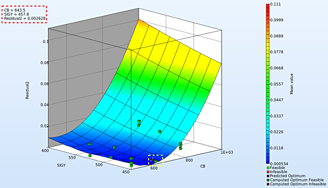
- Note : The surface plot for Residual2 shows a non-linear surface, although we used linear polynomials. The reason is that Curve Mapping is defined as a composite expression that is calculated using the metamodels of the components, and the expression is non-linear.
- The optimum values for the input variables can be visualized in the top-left hand corner, whereas the location of the optimum values on the surface plot can be seen with the purple cross.
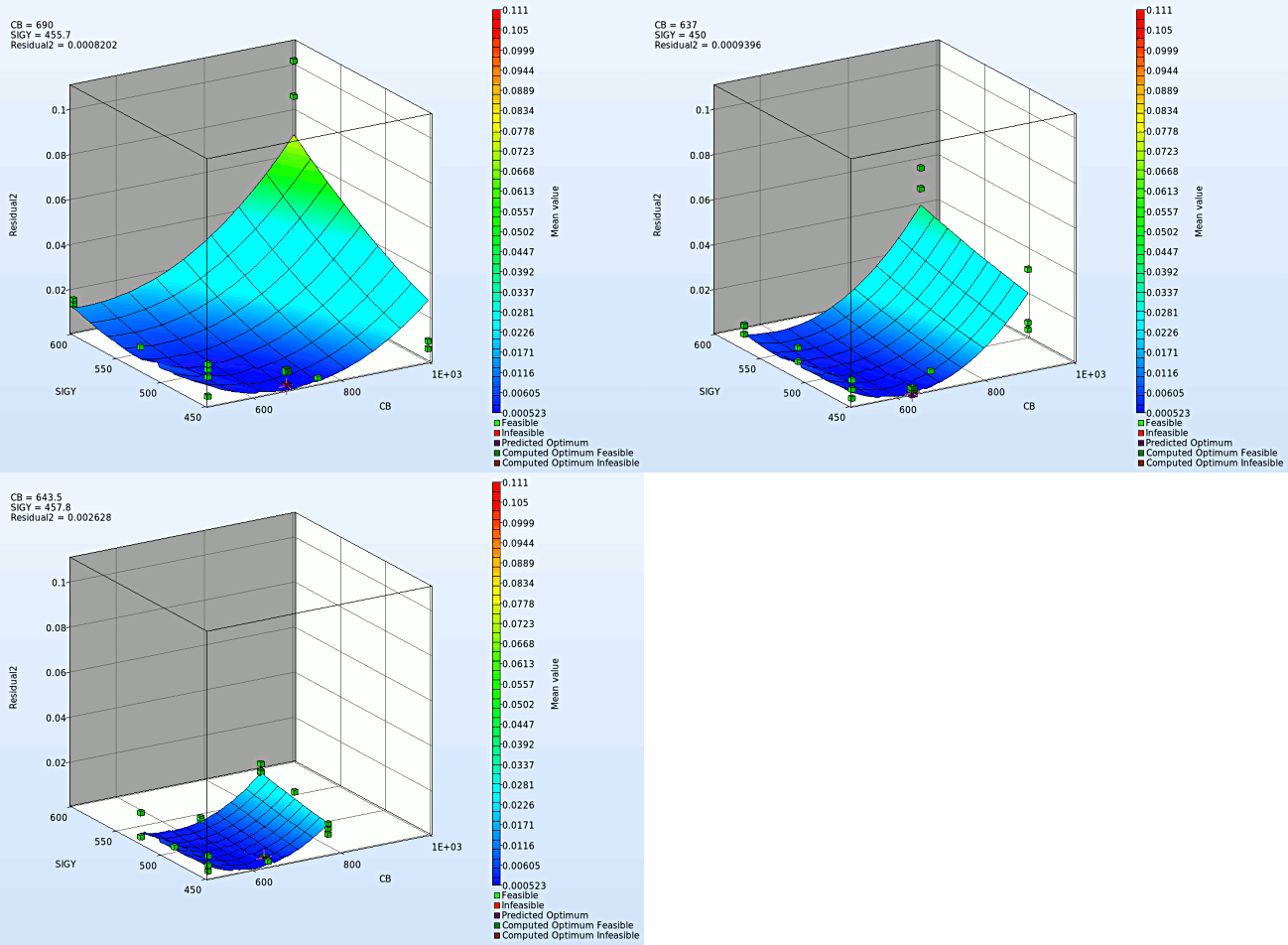
- We rotate the plot with the mouse by pressing Ctrl at the meantime. We can change the surface plot for each iteration (at step 2.) and visualize the effect of domain reduction (as shown below).


