Results
Home Screen Process Flowchart
- The results can be viewed by selecting the view button on the task bar. A seperate window of LS-OPT Viewer opens up.
LS-OPT Viewer
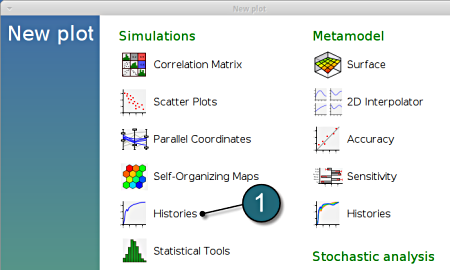
- Select under Simulations the item Histories.
Plot Setup
Setup the plot for pct2
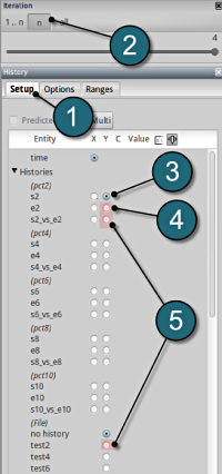
- Select the Setup tab.
- Select n for the iterations setup.
- Plot co-ordinate selections :
x axis : time
y axis : s2
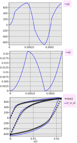
- The first plot in the image depicts a plot of the stress against time.
- In the similar way plot the strain curve by changing the y axis entity to e2.
- The loading cycle curve can be illustrated using the choice for the y axis as s2_vs_e2 and test2. We can notice the hysteresis for the cyclic loading case.
Multiple Plots
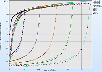
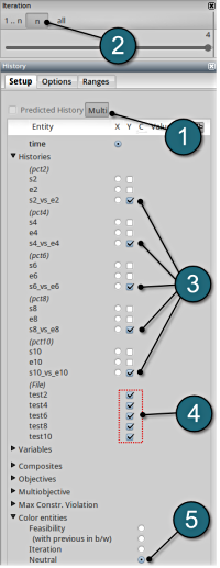
- Select the Multi option to view all the simulation crossplots and test curves simultaneously.
- Select n for the iterations setup and select the last iteration to display the optimal curves.
- To view all the stress-strain crossplots viz. s2_vs_e2, s4_vs_e4, etc. select the respective boxes.
- Similarly select all the test curves viz. test2, test4, etc.
- To distinguish between the crossplots it's convinient to select the Neutral option for the Color entities.
Convergence
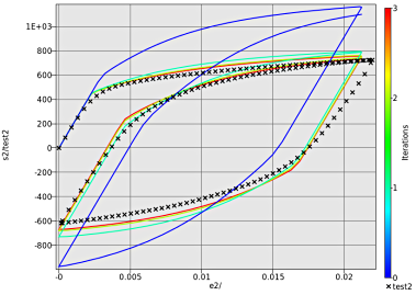
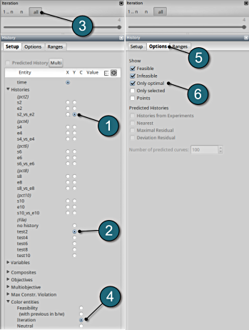
- Select any of the history curves. In this case s2_vs_e2 plot has been selected.
- From the file histories select the corresponding test curve, e.g. test2.
- To observe the convergence over the iterations choice is made for all the iterations.
- To distinguish between the iterations choice of Color entities is made on the Iterations.
- Select the Options tab.
- To show the optimal curves over the iterations the Only optimal option has been selected.
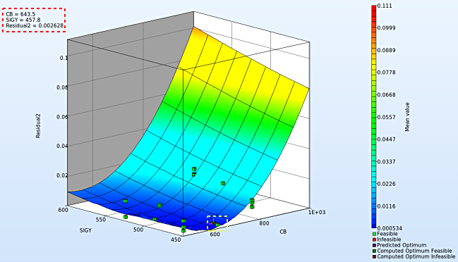
We can plot the several surface plots of the metamodel we've built. For example, we want to see a surface plot of the objective function Residual2 with respect to the variables CB and SIGY, do it as following:
New Plot
- To view a new plot select the plot button on the task bar. A seperate window of LS-OPT Viewer opens up.
LS-OPT Viewer
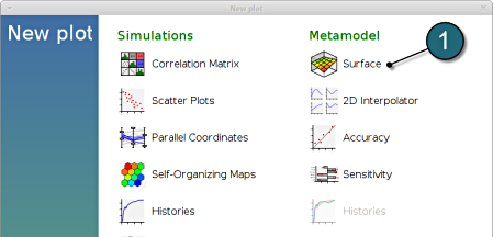
- Select under Metamodel the item Surface.
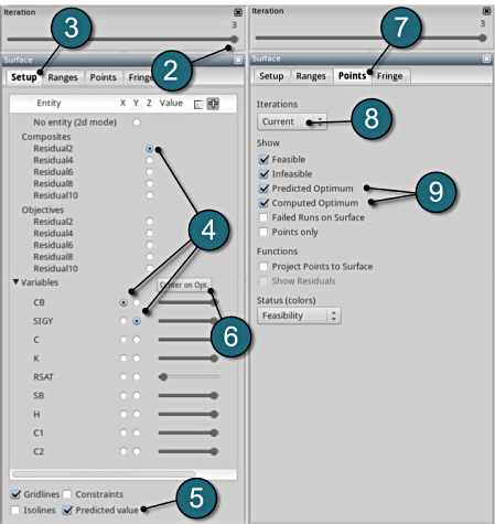
- Slide to the last iteration.
- Select the Setup tab.
- Set Residual2 as the z-coordinate, the variables CB and SIGY as the x-coordinate and y-coordinate, respectively.
- Choose Predicted value. A purple cross will appear somewhere on the surface. You can move it by changing the values of the variables CB and SIGY using the respective sliders. The predicted value for the selected parameter combination is displayed.
- Click Center on Opt. to locate the cross at the optimal point.
- Select the Points tab.
- Make the selection for Iterations at Current.
- Pick Predicted Optimum and Computed Optimum.
- In the similar way, we can visulaize the metamodel surface for the other Composites / Objectives with respect to the input parameters.
- Note : The surface plot for Residual2 shows a non-linear surface, although we used linear polynomials. The reason is that Curve Mapping is defined as a composite expression that is calculated using the metamodels of the components, and the expression is non-linear.
- The optimum values for the input variables can be visualized in the top-left hand corner, whereas the location of the optimum values on the surface plot can be seen with the purple cross.
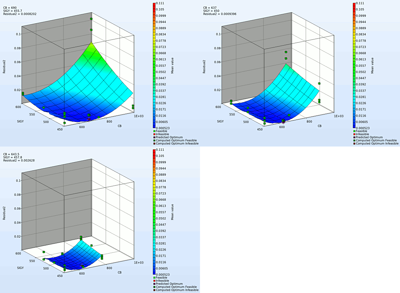
- We rotate the plot with the mouse by pressing Ctrl at the meantime. We can change the surface plot for each iteration (at step 2.) and visualize the effect of domain reduction (as shown below).
Fig. Effect of domain reduction on optimization process
What is the approximation error of the result?
The approximation error indicators (predict the metamodel accuracy of the results) can be visualized in the LS-OPT Viewer.
New Plot
- To view a new plot select the plot button on the task bar. A seperate window of LS-OPT Viewer opens up.
LS-OPT Viewer
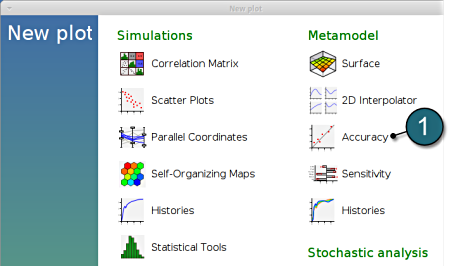
- Select under Metamodel the item Accuracy.
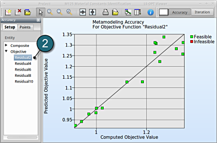
- From Entity select the Objective Residual2.
→ Good approximation: low distance between black line and green points.
→Similar observations can be made by selecting the other objectives.
Optimization History
- Alternatively the accuracy of the optimal values at various iterations can be studied under a Optimization History plot.
New Plot
- To view a new plot select the plot button on the task bar. A seperate window of LS-OPT Viewer opens up.
LS-OPT Viewer
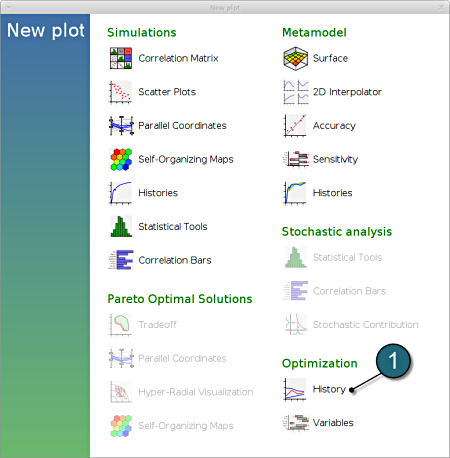
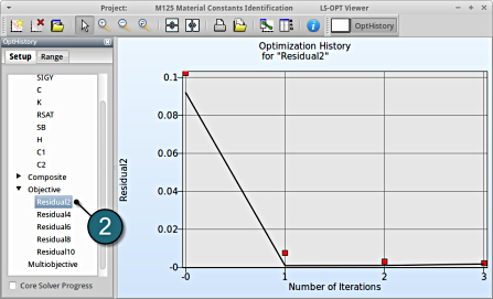
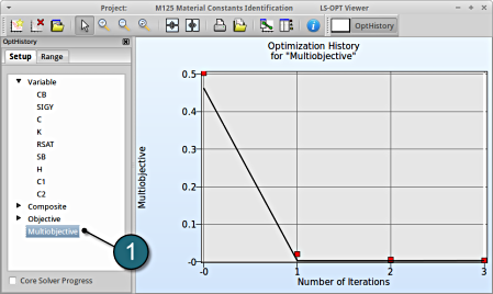
- Select under Optimization the item History.
- From Setup tab, select the Objective Residual2.
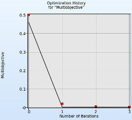
→ Good approximation of optima: The computed values (red points) almost coincide with the predicted values (black line) for the optimum.
→Similar observations can be made by selecting the other objectives.
→For observing the multiobjective select the option.
New Plot
- To view a new plot select the plot button on the task bar. A seperate window of LS-OPT Viewer opens up.
LS-OPT Viewer
- Choose History under the category Optimization.
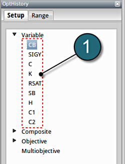
We can choose from the left side the entities we want to observe.
Convergence of Input variables
Setup
- Select the input variable to observe the convergene behaviour across the iterations.
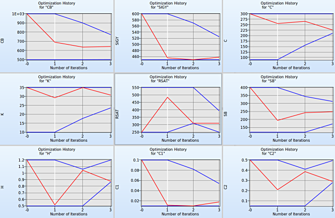
Use the split plot from the task menu to compare the various Optimization Histories of the input variables. Interesting revelations can be made from the plots. (Shown in figure below)
Fig. Convergence behaviour of all input variables.
Convergence of Objectives
1. Select Objective → Multiobjective
- The predicted result (black line) of the optimal objective Multiobjective for every iteration.
- The computed result (red points) of the optimal objective Multiobjective for every iteration.
- The convergence trend of the Multiobjective.
Which variable appears to be the most important?
The significance of a variable for a response can be illustrated with ANOVA (analysis of variance) or GSA/Sobol (global sensitivity analysis). In this case, only GSA is available, since ANOVA is only calculated for responses, not for composites.
New Plot
- To view a new plot select the plot button on the task bar. A seperate window of LS-OPT Viewer opens up.
LS-OPT Viewer
GSA/Sobol
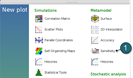
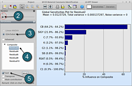
- Restart the LS-OPT Viewer and select under Metamodel the item Sensitivity
- We can slide to observe the sensitivity of results at each iteration. In this case for Iteration 1.
- The linear ANOVA measure is unavailable. Choice can be kept at GSA/Sobol.
- Select any of the Composite to observe the sensitivity measure. In this case select Residual2.
- Select Sort for the variables.
→ For the composite Residual2 the variable CB is the most important or significant, followed by the variable SIGY.
→ Similar observation can be made for the other composites upon selection.
Multiple Responses Sensitivity
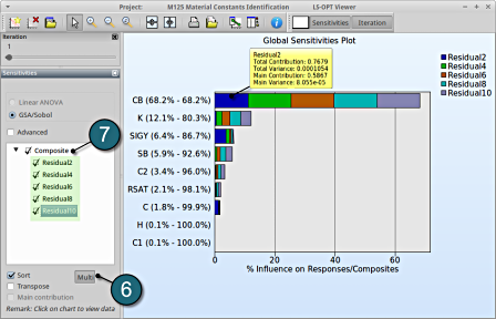
The viewer allows the user to select multiple responses and composites for sensitivity analysis to get the influence of the variables on e.g. the whole problem or a load case using the following steps:
- Select the Multi option.
- Select the desired entities, in this case all the composites are selected .
- The plot describes the cumulative values on a single graph w.r.t. the variables. This is only availabe for GSA, since the values are normalized.

