Parameter Identification

System parameter identification is a commonly used feature of LS-OPT, especially for the purpose of calibrating material models.

The procedure consists of minimizing the mismatch between target values and corresponding solver output values, or between two curves. In the latter case, the two curves typically consist of a two-dimensional experimental target curve and a computed curve. The computed curve is a variable response, being dependent on the system parameters, e.g. material constants. It can also be a crossplot, constructed by combining two time histories such as strain and stress.

The two main essential components of an algorith designed for system identification are

→ optimization algorithm and

→ curve matching metric

Optimization algorithm

The recommended optimization algorithm to be used to solve a parameter identification problem is the Metamodel-based Optimization with the strategy Sequential with Domain Reduction. Use linear polynomial metamodels and D-optimal point selection which is the default for the selected task and strategy.

Matching scalar values

To match scalar values, extract the respective responses from the solver output. Specify a Standard Composite of type MSE or Sqrt MSE and using these responses as components associated with the respective target value. Define this composite as an objective function.

Curve matching metric

To calculate the mismatch between the target and the computed curve, define a Curve Matching composite. There are two curve matching metrics available, Mean Square Error and Curve Mapping. Mean Square Error is an ordinate-based curve matching metric. Hence if the curve has steep parts or if the ordinate values are not unique, (the curve is a hysteretic curve), Curve Mapping is the metric of choice.
Because Curve Mapping uses the length of the curve to calculate the mismatch, filtering of the component history curves is recommended.

Sampling constraints

For parameter identification problems, there are often more restrictions on design variables than just a lower and an upper bound for each parameter, e.g. there may be a requirement to obtain monotonically increasing solver input curves. Such constraints can be defined as Sampling Constraints in LS-OPT.

Parameterization of solver input curves

A common way to parameterize a solver input curve is to use a parameterized analytical function that represents the characteristic of the curve. Use a program or script as a solver of a preprocessor stage to calculate the solver input curve depending on parameters.
 

Viewer

Some of the postprocessing options commonly used for parameter identification problems are as follows.

Optimization History

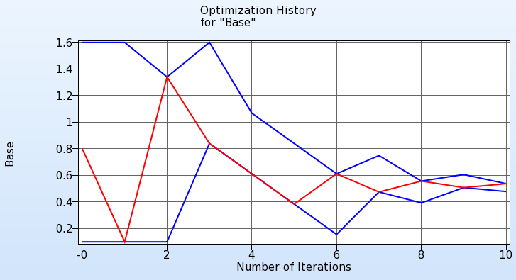
The optimization history plot can be used to check the convergence of the variable values as well as the decrease of the objective over the iterations.

Sensitivities

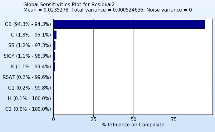
If there are parameter that do not converge, the sensitivities plot can be used to see if those parameters are insensitive.

History

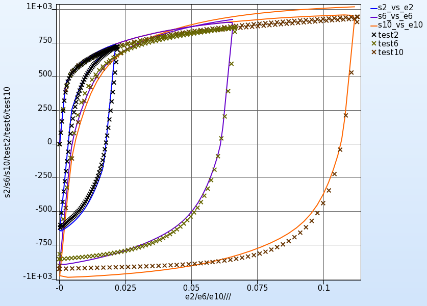
The history plot can be used to display the computed curves and the test curve in the same plot.

There are several coloring options for the computed curves, e.g. the curves could be colored by the objective values (curve matching metric) to see if the curve matching metric works as expected.

Displaying the curves for all iterations, selection the option Only optimal and coloring the curves by iteration visualized the improvement of the optimal curves over the iterations.