Strategies for metamodel-based optimization
Single Iteration
In this approach, the experimental design for choosing the sampling points is done only once. A typical application would be to choose a large number of points (as much as can be afforded) to build metamodels such as, RBF networks using the Space Filling sampling method. This is probably the best way of sampling for Space Filling since the Space Filling algorithm positions all the points in a single cycle.
Required settings:
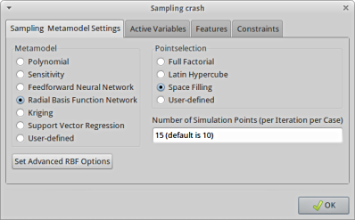
- Use RBF networks or FF neural networks. RBF is the default since RBF networks are much quicker and in some cases more accurate than FF networks.
- Select the number of sampling points.
The following options should default to the settings indicated:
- Space Filling sampling.
The GUI settings are also explained in Figure 20.1.
Figure 20.1 Required settings in Sampling panel for Single Stage strategy
Sequential strategy
In this approach, sampling is done sequentially. A small number of points is chosen for each iteration and multiple iterations are requested. The approach has the advantage that the iterative process can be stopped as soon as the metamodels or optimum points have sufficient accuracy. It was demonstrated that, for Space Filling, the Sequential approach had similar accuracy compared to the Single Stage approach,i.e. 10 × 30 points added sequentially is almost as good as 300 points. Therefore both the Single Stage and Sequential Methods are good for design exploration using a surrogate model. For instance when constructing a Pareto Optimal Front, the use of a Single Stage or Sequential strategy is recommended in lieu of a Sequential strategy with domain reduction (see Sequential strategy with domain reduction).
Both the previous strategies work better with metamodels other than polynomials because of the flexibility of metamodels such as neural networks to adjust to an arbitrary number of points.
Required settings:
- Choose either RBF networks or FF neural networks. RBF is the default, since RBF networks are much quicker and in some cases more accurate than FF networks.
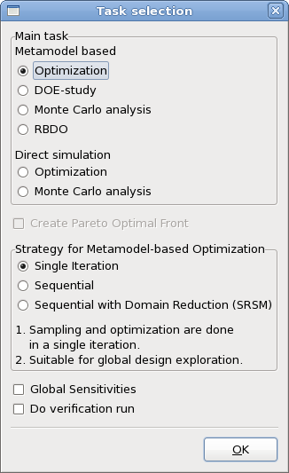
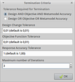
- Adjust the iteration limit in the Termination Criteria dialog.
The following options should default to the settings indicated:
- Space Filling sampling.
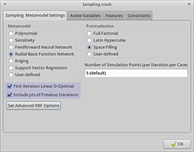
- The first iteration is Linear D-Optimal.
- Use adaptive sampling. This implies that the positions of points belonging to previous iterations are taken into account when choosing new Space Filling points. Metamodels are also built using all available points, including those of previous iterations. The GUI check box is “Include pts of Previous Iterations”.
- Choose the number of points per iteration to not be less than the default for a linear approximation ( 1.5(n + 1)).
The GUI settings are also explained in Figure 20.2.

Figure 20.2 Required settings in Sampling panel (left) and Run panel (right) for sequential strategy without domain reduction
Sequential strategy with domain reduction
This approach is the same as the Sequential strategy but in each iteration the domain reduction strategy is used to reduce the size of the subregion. During a particular iteration, the subregion is used to bound the positions of new points. This method is typically the only one suitable for polynomials. There are two approaches to Sequential Domain Reduction strategies. The first is global and the second, local.
Sequential Adaptive Metamodeling (SAM)
As for the Sequential strategy without domain reduction, sequential adaptive sampling is done and the metamodel constructed using all available points, including those belonging to previous iterations. The difference is that in this case, the size of the subregion is adjusted (usually reduced) for each iteration. This method is good for converging to an optimum and moderately good for constructing global approximations for design exploration such as a Pareto Optimal front. The user should however expect to have poorer metamodel accuracy at design locations remote from the current optimum.
Required settings:
- Choose either RBF or FF neural networks. RBF networks are much quicker than FF networks. RBF networks have shown some sensitivity to domain reduction methods.
- Set the iteration limit in the Termination Criteria dialog.
The following options should default to the settings indicated:
- Space Filling sampling.
- Choose the number of points per iteration to not be less than the default for a linear approximation ( 1.5(n + 1) ).
- Check the box for the first iteration to be Linear D-Optimal.
- Use adaptive sampling. This implies that the positions of points belonging to previous iterations are taken into account when choosing new Space Filling points. Metamodels are also built using all available points, including those of previous iterations.
In the GUI, the sampling panel setting is the same as in Figure 20-2 (left).
Sequential Response Surface Method (SRSM)
SRSM is the original LS-OPT automation strategy and allows the building of a new response surface (typically linear polynomial) in each iteration. The size of the subregion is adjusted for each iteration. Points belonging to previous iterations are ignored. This method is only suitable for convergence to an optimum and should not be used to construct a Pareto optimal front or do any other type of design exploration. Therefore the method is ideal for system identification.
Required Settings:
- Set the maximum number of iterations in the Termination Criteria dialog.
The following options should default to the settings indicated:
- Metamodel type Linear polynomial
- D-optimal point selection
- Default number of sampling points (50% oversampling).


