Curve Matching Metrics
Background
One popular use of LS-OPT is for identifying system parameters; for instance material properties. This is typically done by having one or more curves from a physical experiment. The experiment is then duplicated in LS-DYNA, and LS-OPT is used for trying to find the appropriate parameters that will generate a curve similar to the one in the experiment.
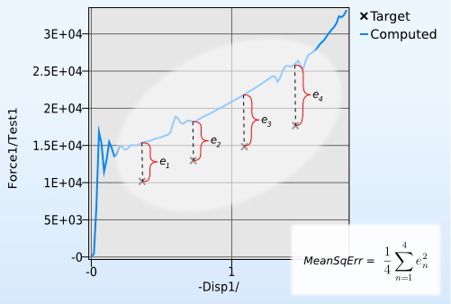
In order to set up an optimization problem for parameter identification, some kind of error measure between curves is needed so that LS-OPT has something to minimize. The classic LS-OPT curve error measure is the MeanSqErr composite, illustrated by Figure 1.

Figure 1: How the MeanSqErr error is calculated. Points in the target curve have their y-value compared to interpolated points in the calculated curve
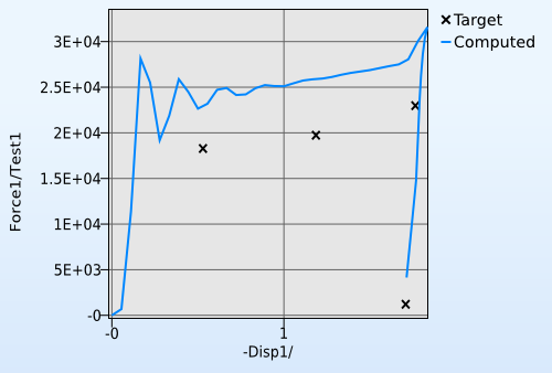
The MeanSqErr approach has some obvious drawbacks. For instance, it requires a history curve with monotonously increasing x-value. This rule gets broken for instance in the case of a force-displacement curve where the force exerted on the specimen disappears at a specific point in time. This is illustrated by Figure 2.

Figure 2: Plot of a curve that would stump MeanSqErr
Enter Curve mapping, another approach to curve error measurement in LS-OPT. Instead of just looking at curve Y values, this method uses the area of the polygon one would get by drawing the target curve, followed by a segment of the calculated curve in reverse, then closing the polygon by returning the starting position.
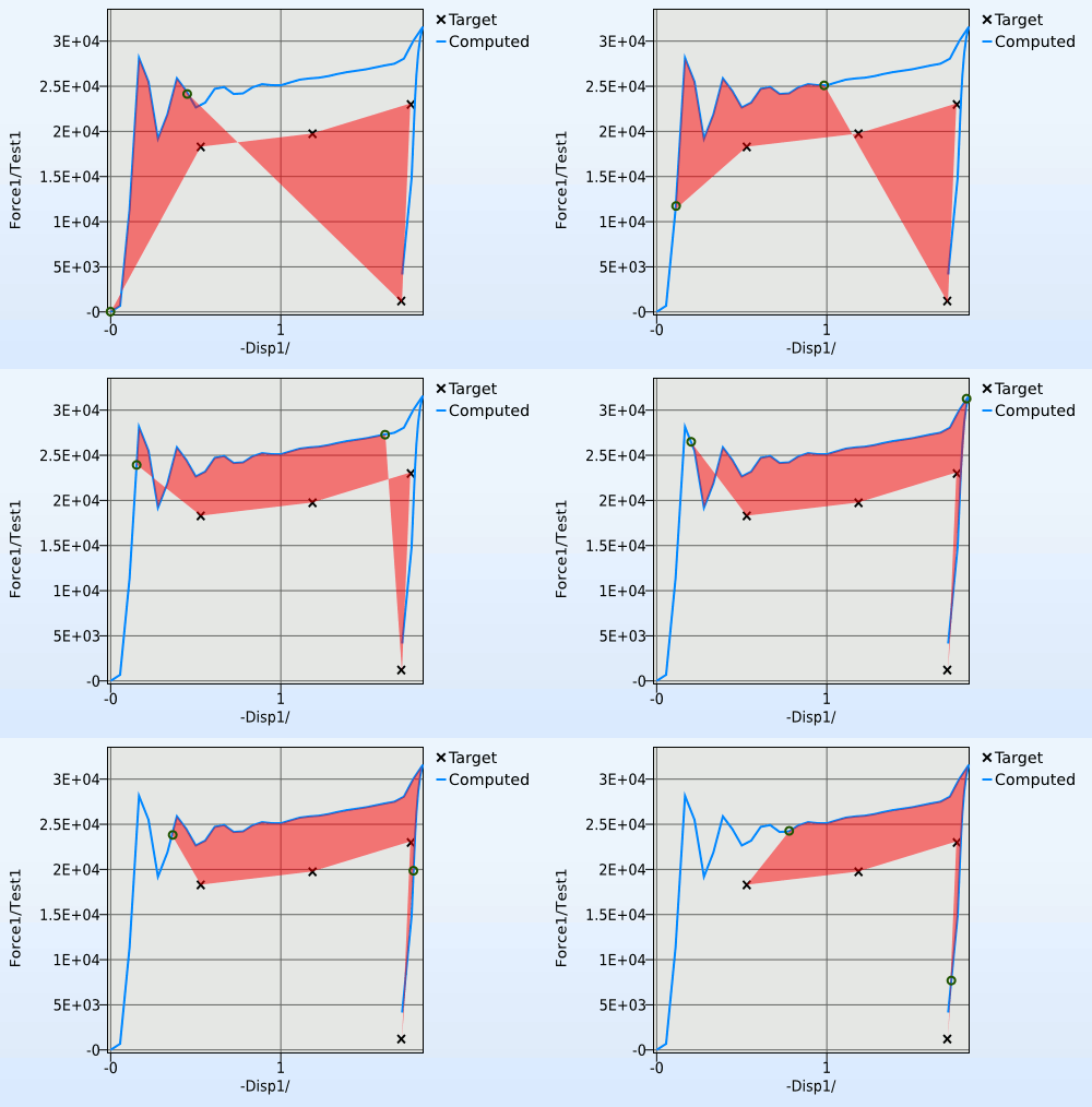
There is an obvious problem with this method: how to determine which part of the calculated curve to compare with the target curve. This is done by starting at the first point of the computed curve, and creating a segment with the same length as the target curve. This segment is then pushed forward along the computed curve in order to find the segment that would create the smallest polygon. An attempt to illustrate this is the animation in Figure 3.

Figure 3: The curve mapping segment finder illustrated.
All of this happens in normalized space to avoid biases when axis scales are of different magnitude.
At this point you might ask: are there any drawbacks to using Curvemap instead of MeanSqErr? Well, the MeanSqErr algorithm might perform better than Curvemap when the computed curve and the target curve have significantly different bandwidth. This happens because a curve with high frequencies is geometrically longer than a filtered curve, thus messing up the curve segment matching. However, even MeanSqErr might perform badly in this case, so always make sure to apply an appropriate filter to the computed curves you extract.
Examples
Further information
An Effective Curve Matching Metric for Parameter Identification Using Partial Mapping
