Linear Sensitivity Analysis
Working Directory and Extraction of necessary files
- Create a working directory in the desired location to keep the LS-OPT project file and input files, as well as the LS-OPT program output, e.g. full_vehicle_model.
- Extract all the files required for this example from download section into the working directory.
Project Details
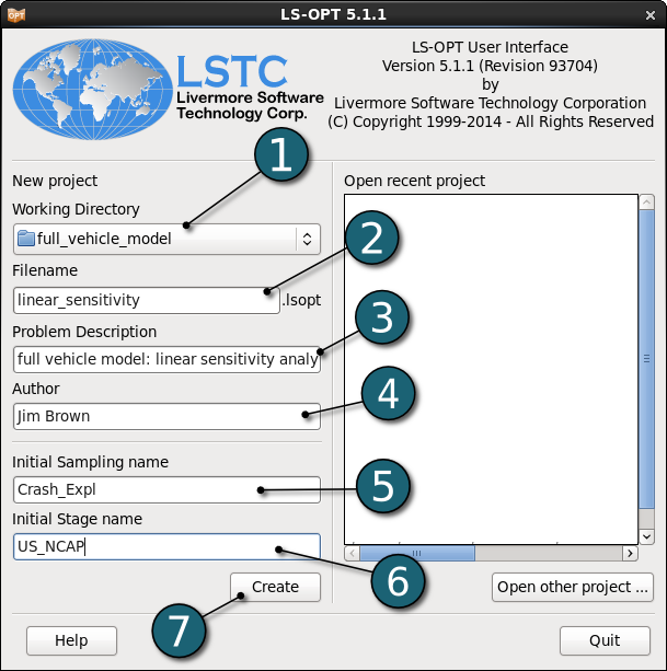
- Select the Working Directory of the LS-OPT project.
- Select a suitable name for the file under Filename (e.g. linear_sensitivity). The extension .lsopt is appended by LS-OPT.
- Description of the main task can e.g. be a suitable name for Problem Description ( in this case, full vehicle model: linear sensitivity analysis, optional) .
- Input the name of the Author (optional).
- Choose a suitable name under the Initial Sampling name (e.g. Crash_Expl).
- Choose a suitable name under the Initial Stage name (e.g. US_NCAP).
- Press the Create button to initiate the formation of the input file.
- The main GUI window of LS-OPT opens.
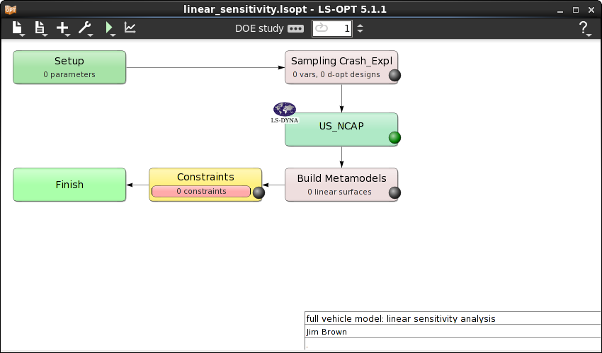
Home Screen Process Flowchart
-
Select the Task icon.
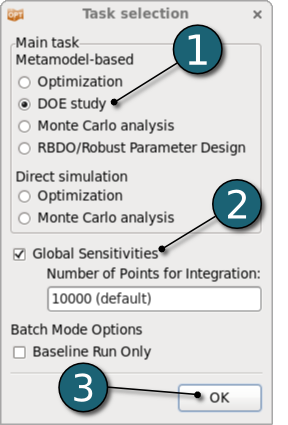
A window Task selection shall open.
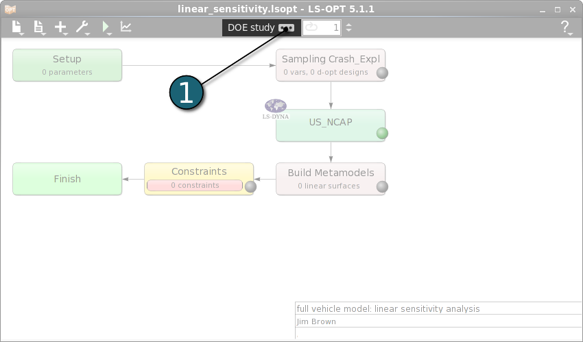
Define the Main Task
- Select the radio button DOE Study for the selection of the main task.
- To study the Global Sensitivities for the input parameters, which is required for sensitivity analysis of this example, tick the adjacent box.
- Push the OK button to proceed.
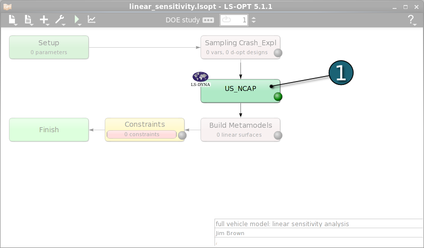
In order to complete the Process Flowchart and before defining further settings in e.g. Setup, Sampling and Constraints, all the load cases that are considered in this sensitivity analysis (US_NCAP, IIHS, Torsion and EVA) are constructed.
Home Screen Process Flowchart
- Double click on the US_NCAP box.
Define Input File Name and Command for US_NCAP
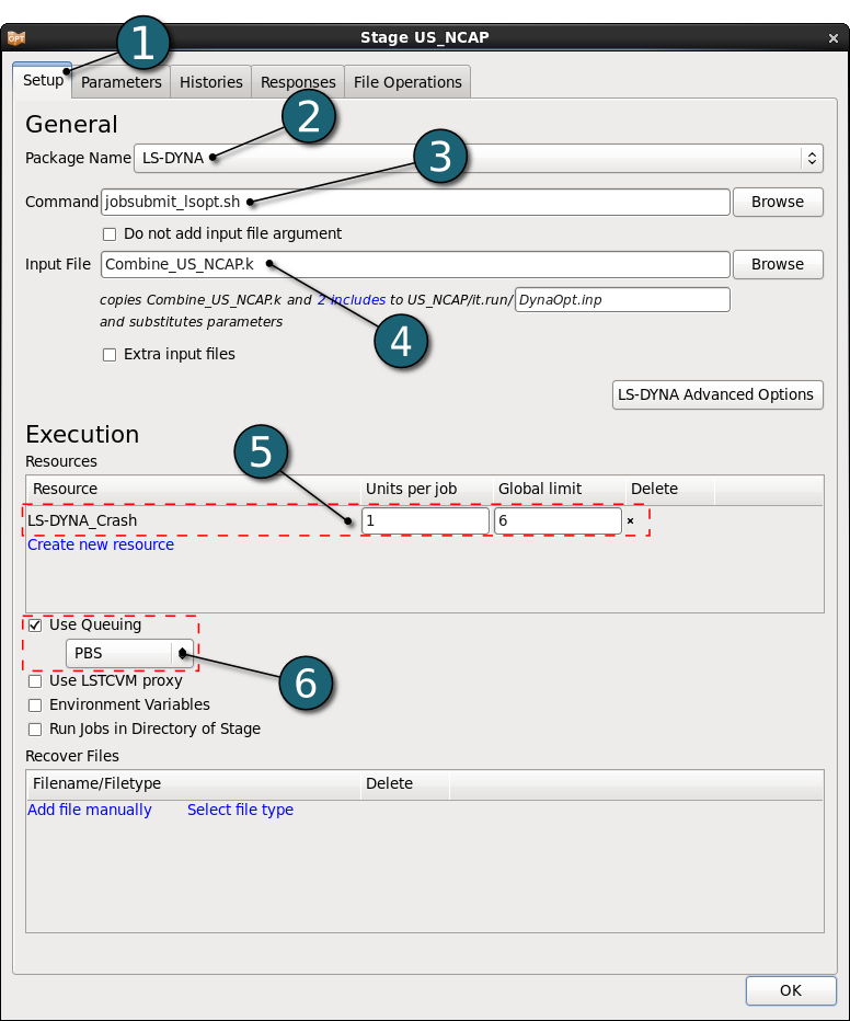
- Select the Setup tab.
- Select the Package Name LS-DYNA.
- For Command specify jobsubmit_lsopt.sh (This is a script that submits the LS-DYNA jobs to a cluster and needs to be replaced by an appropriate command available on your system).
- For Input File browse the parameterized file Combine_US_NCAP.k. Parameters are defined using *PARAMETER.
- For efficient usage of the computing power from the machine, choice on handling number of concurrent jobs can be made suitably in this section. For more details see FAQ resources.
- In case you run the LS-DYNA jobs on a cluster, activate Use Queuing and select the respective queuing system, e.g. PBS, for interfacing with load sharing facilities to enable running simulation jobs across a network.
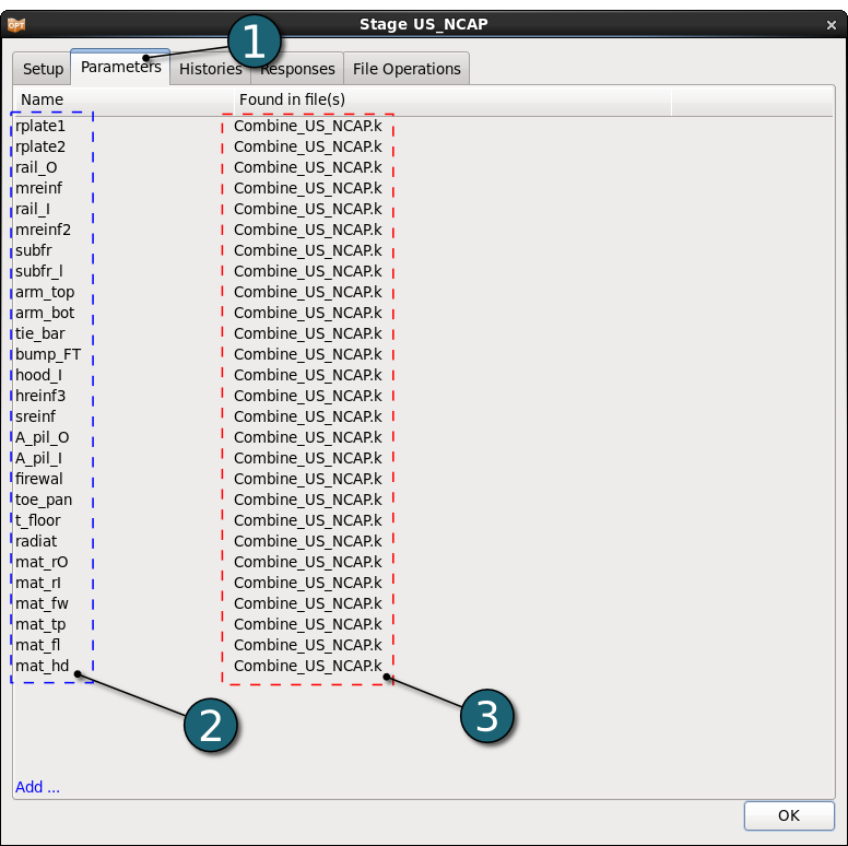
The parameters defined in the selected Input File can be visualized in the adjoining tab Parameters.
Design Parameters for Crash Case.
|
.
...
$ ===============
$ PARAMETER cards
$ ===============
$
*PARAMETER
R rplate1 2.51
R rplate2 1.52
R rail_O  1.91
R mreinf  2.55
R rail_I  1.9
R mreinf2 2.4
R subfr   2.25
R subfr_l 2.25
R arm_top 2.25
R arm_bot 2.25
R tie_bar 4.3
R bump_FT 2.85
R hood_I  .8
R hreinf3 1.22
R sreinf  2.5
R A_pil_O 1.4
R A_pil_I 2.
R firewal .75
R toe_pan 1.9
R t_floor .8
R radiat  3.6
I mat_rO  270
I mat_rI  270
I mat_fw  270
I mat_tp  300
I mat_fl  270
I mat_hd  240
...
.
|
Define the Histories for Crash Load Case US_NCAP
Histories are vectorial output entities of the simulations, e.g. displacement over time curves. Histories may be used to calculate scalar output entities, e.g. the maximal displacement.
Define x-acceleration of nodes:
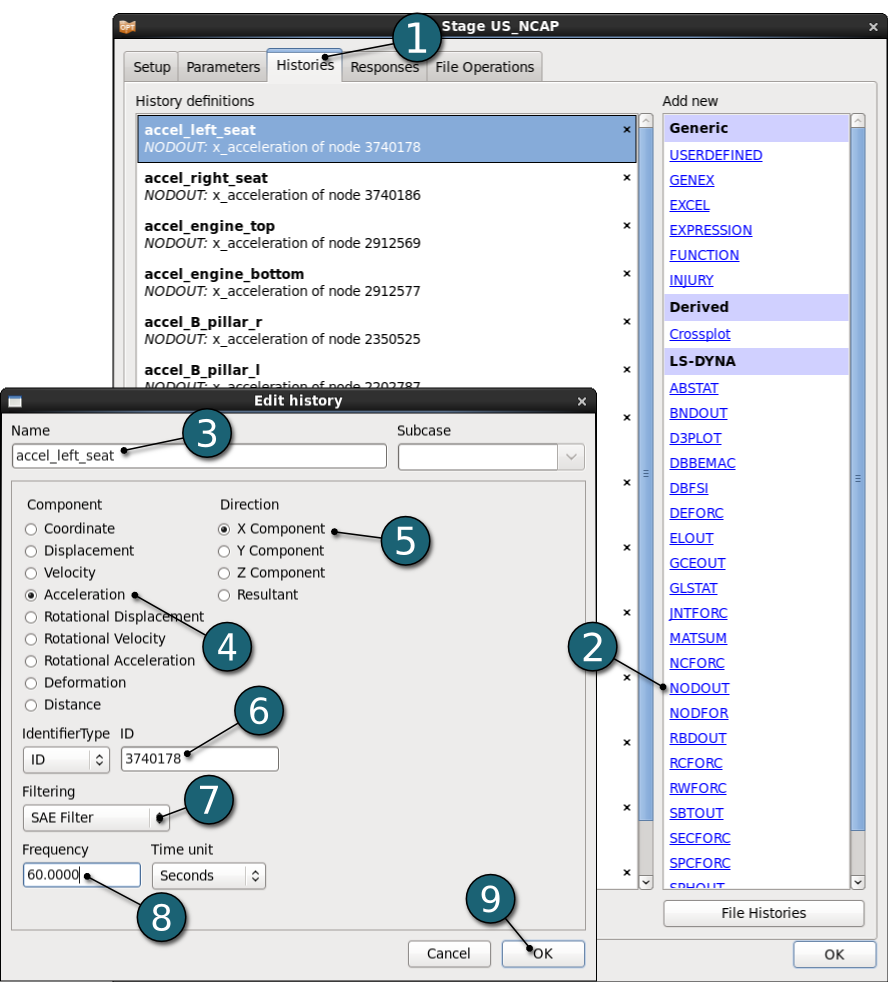
- Select the Histories tab.
- Select NODOUT history type from the various option available from the list under Add new. A separate window emerges named Edit history. This enables the user to define the history in suitable steps.
- For History Name enter accel_left_seat.
- For Component select from the list Acceleration.
- For Direction select X Component.
- For Node ID enter 3740178.
(The acceleration of the left seat is measured at node 3740178. To see the position of the node click on the ID-number.) - For Filtering choose SAE Filter.
- Enter 60.0 for Frequency.
- Click on the OK button to proceed.
For the rest of the Acceleration Histories ( e.g. accel_right_seat, accel_engine_top, accel_engine_bottom, accel_B_pillar_r, accel_B_pillar_l ) repeat the steps 2 to 9 or copy the previously defined history, updating only the Node IDs and Names.
Define Intrusion
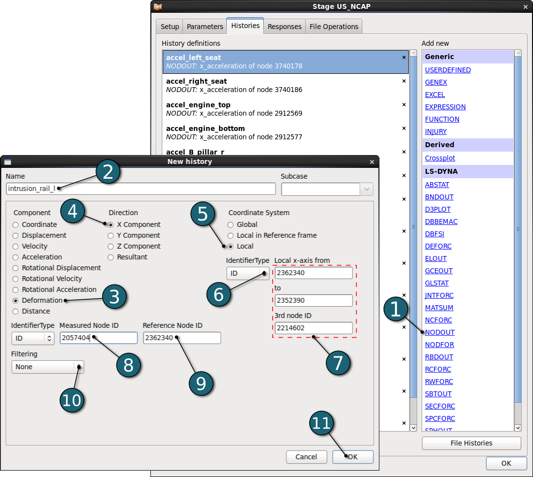
- From the LS-DYNA interfaces select: NODOUT.
- For History Name enter intrusion_rail_l.
- For Component select from Deformation.
- For Direction select X Component.
- For Coordinate System select Local.
- For Identifier Type switch to ID.
- Enter for Local x-axis from 2362340 to 2352390, 3rd node ID 2214602.
- For Measured Node ID enter 2057404. To see the position of a node click on the ID number.
- For Reference Node ID enter 2362340.
- For Filtering choose None.
- Click on the OK button to proceed.
For the rest of the Intrusion-Histories ( e.g. intrusion_rail_r, intrusion_break_pedal, intrusion_gas_pedal, intrusion_steering, intrusion_firewall_left, intrusion_firewall_right) repeat the steps 1 to 11 or copy the previously defined history, updating only the Measured Node IDs and Names.
Define an Expression
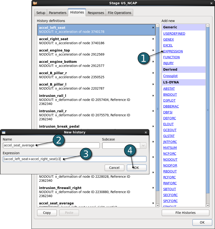
- In order to calculate the average acceleration of a seat the predefined histories accel_left_seat and accel_right_seat will be used. The average acceleration of a seat will then be defined as an expression.
- From the possible history types select: EXPRESSION.
- For History Name enter accel_seat_average.
- In the input field for an algebraic expression enter (accel_left_seat+accel_right_seat)/2.
- Click on the OK button to proceed.
Define the Responses for Crash Load Cases US_NCAP
Define mass:
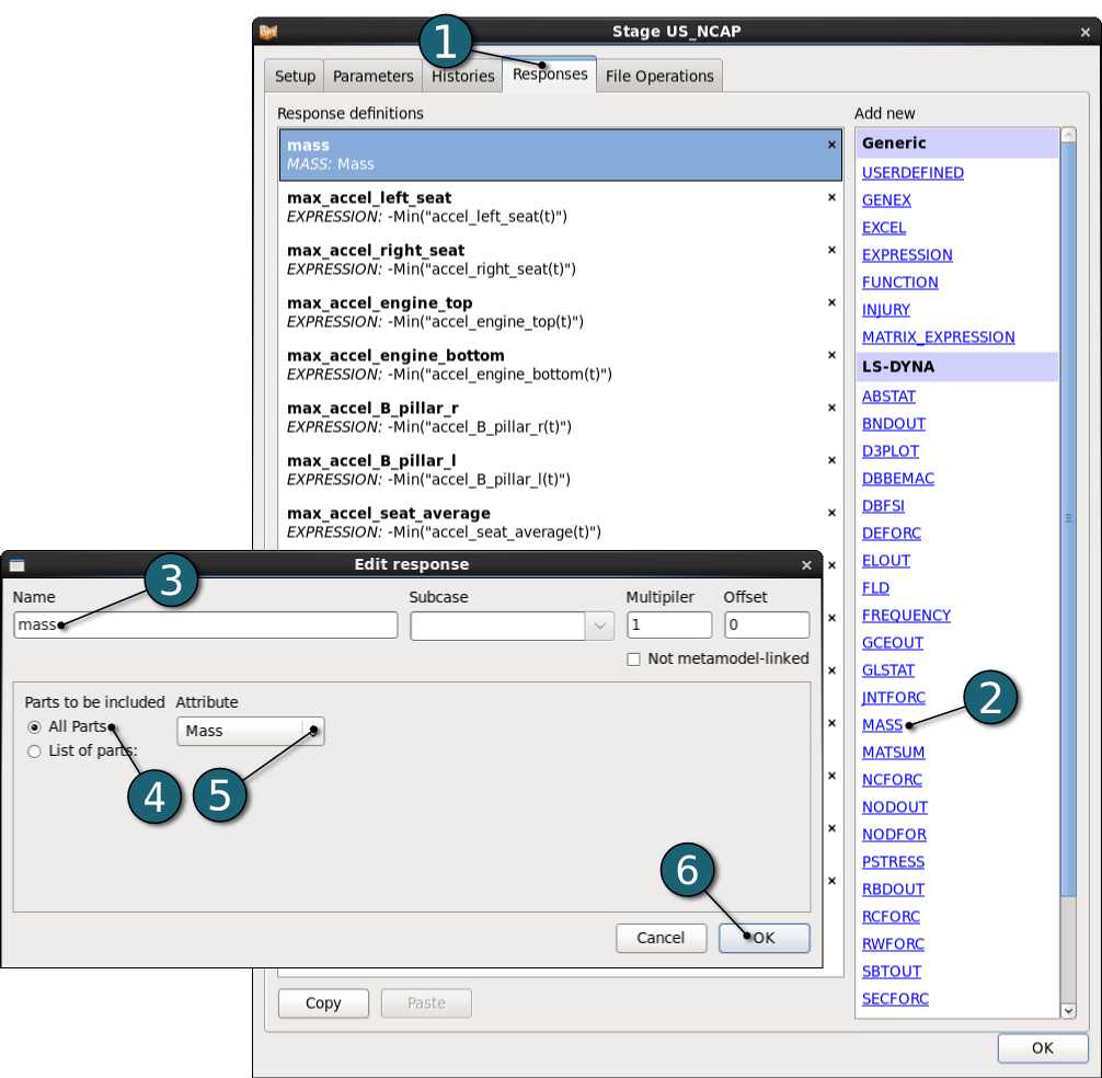
- Select the Responses tab.
- From the LS-DYNA interfaces select: MASS.
- For Response Name enter mass.
- For Parts to be included select All Parts. This will extract the mass of the full model.
- For Attribute choose Mass.
- Click on the OK button to proceed.
Define maximum acceleration
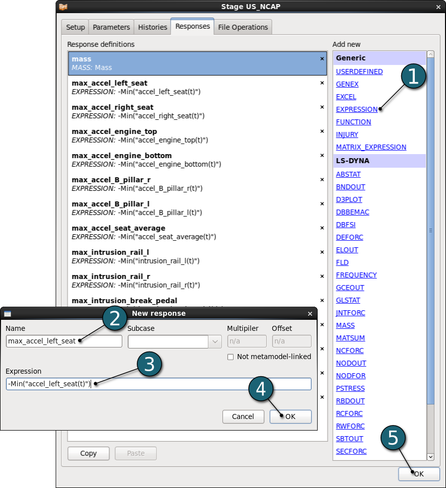
- From the possible response types select: EXPRESSION.
- For Response Name enter max_accel_left_seat.
- For Expression enter: -Min("accel_left_seat(t)").
(To define the expressions we can use here histories, that we defined in the Histories tab.)
Since the x-axis is defined in opposite direction of motion, we have to define the expressions for maximum as "-minimum". - Click on the OK button to continue.For the rest of the maximum acceleration-responses ( e.g. max_accel_right_seat, max_accel_engine_top, max_accel_engine_bottom, max_accel_B_pillar_r, max_accel_B_pillar_l ) repeat the steps 1 to 5 or copy the previously defined response, updating the algebraic expressions and Names.
The same applies to responses for maximum intrusion. - Click on the OK button to finish to define the Crash load cases, e.g. US_NCAP.
Cloning Stages
Since the histories and responses are identical for both US_NCAP and IIHS load cases, the Clone option may be used to create the load case IIHS from the already defined US_NCAP stage:
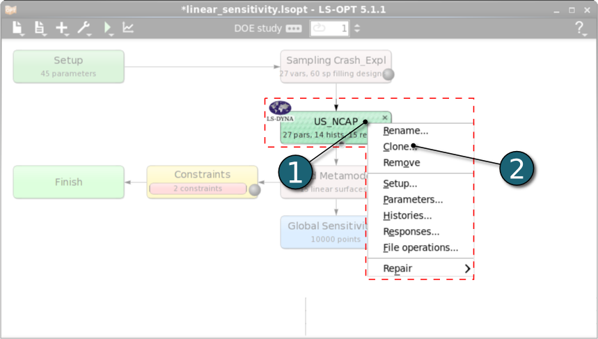
- Right click on the Stage US_NCAP box on the main GUI.
- Select the option Clone.
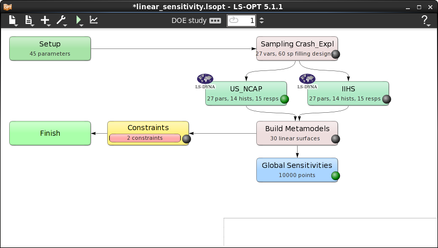
Enter the name of the New Stage : IIHS
- A new stage has been created in the main GUI with the same definitions than the basis stage.
- When required the New Stage IIHS can be edited using the similar steps as shown in the previous tabs, but in this example they are identical except that the only thing that have to be changed is the Input File for the IIHS loadcase.
- History and response names are updated automatically by LS-OPT to ensure uniqueness of names.
Adding Sampling
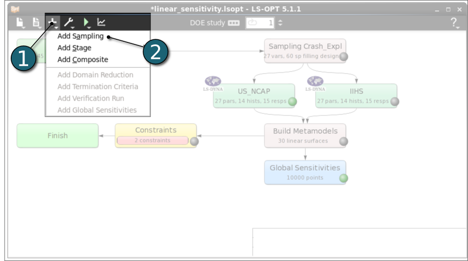
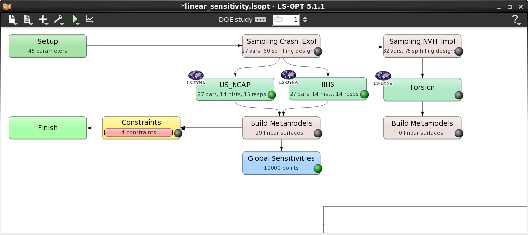
Before continuing with defining the other stages i.e. Torsion and EVA, an additional sampling is added for the implicit NVH and Eigenvalue simulations for the efficiency, since the parameters considered in NVH and Eigenvalue simulations differ from those of the crash simulations.
- Click on the Add option on the control bar on the main GUI.
- Click on the option Add Sampling.
Enter the name of the New Sampling: NVH_Impl.
Adding Stage Torsion
After the Sampling NVH_Impl is created the remaining stages i.e. Torsion and EVA can be added in this sampling.
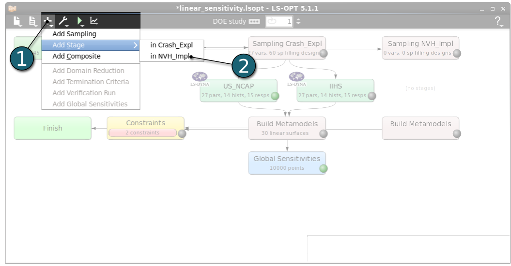
- Click on the Add option on the control bar of the main GUI.
- Under Add Stage option click on the created in NVH_Impl sampling.
Enter the name of the New Stage: Torsion
- A new sampling and stage have been created in the main GUI.
- To define Input File Name and Command of Stages Torsion and EVA and to view the Design Parameters for NVH and Eigenvalue simulations follow the steps under US_NCAP and Param. Tabs.
Add & Define Stage EVA
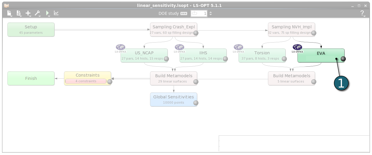
Add Stage EVA
- Click on the Add aption on the control bar on the main GUI.
- Under Add Stage option click on the created in NVH_Impl sampling.
Enter the name of the New Stage: EVA
Define the Stage EVA
Home Screen Process Flowchart
- Double click on the EVA box.
A window Stage EVA shall open.
- In a similar way to Stage Torsion the Input File for the load case EVA for Eigenvalue simulations can be defined.
- There are no Histories defined (vectorial quantities) in this load case because the quantities to be defined are only scalar quantities (responses) e.g. frequency modes.
Define Responses for EVA:
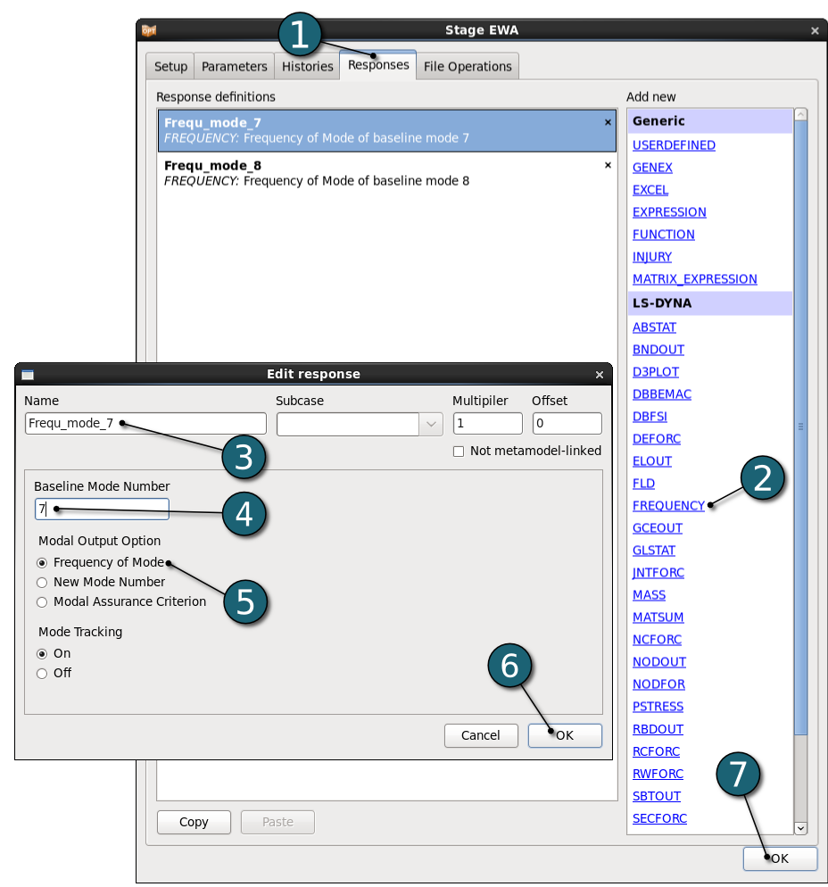
Define Frequency mode 7:
- Select the Responses tab.
- From the LS-DYNA interfaces select: FREQUENCY.
- For Response Name enter Frequ_mode_7.
- For Baseline Mode Number type 7.
- For Modal Output Option select Frequency of Mode.
- Click on the OK button to proceed.
Repeat steps 1 to 6 or copy the previsouly define dresponse for frequency mode 8 only changing Baseline Mode Number to 8.
- Click on the OK button to finish defining Stage EVA.

Home Screen Process Flowchart
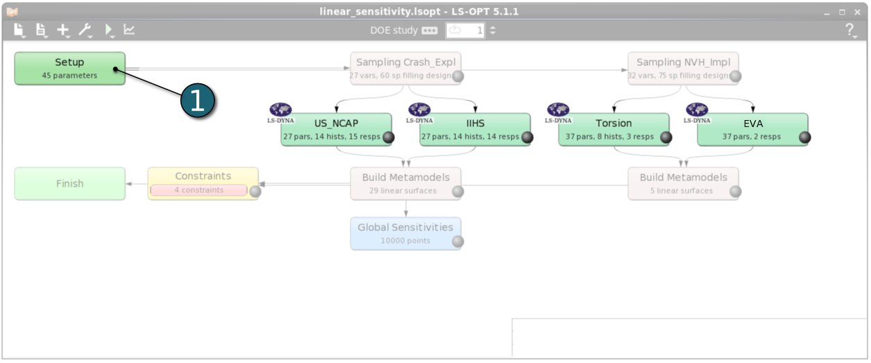
- Double click on the Setup box.
A window Problem global setup shall open.
Define the Parameters:
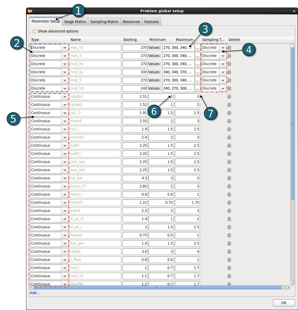
- Select the Parameter Setup tab.
- The first six material variables are discrete variables defining different steel types. So for Type switch the menu to Discrete.
- Enter 270 300 340 370 410 480 800 for the list of allowable Values of the variable mat_rO. The value is the yield stress of the respective material.
- For Sampling Type switch to Discrete.
(For details see FAQs.) - For Type of remaining variables switch the menu to Continuous.
- Enter 2 for the Minimum of the variable rplate1.
- Enter 3 for the Maximum of the variable rplate1.
- Since the parameters are already defined in the input files, they cannot be deleted manually. This is indicated by the lock symbol on the left on Parameter Setup window.
Repeat steps 3 and 4 for the rest of discrete variables, updating the discrete values for each variable.
Repeat steps 6 and 7 for the rest of variables, updating minimum and maximum for each variable.
Stage Matrix
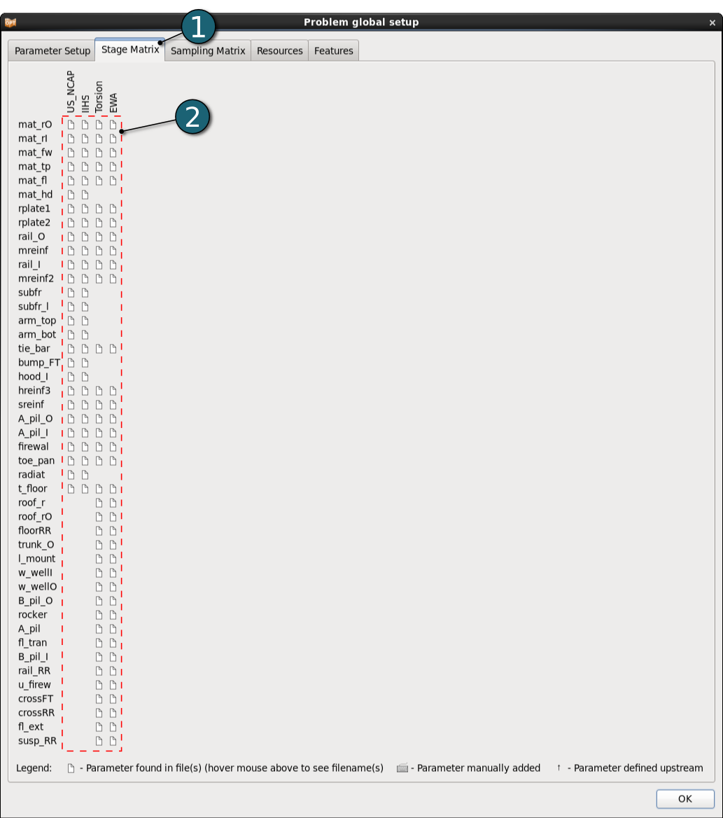
- Select the Stage Matrix tab.
- You find a matrix of parameters vs. stages, and symbols that visualize if parameters are found in input files.
Sampling Matrix
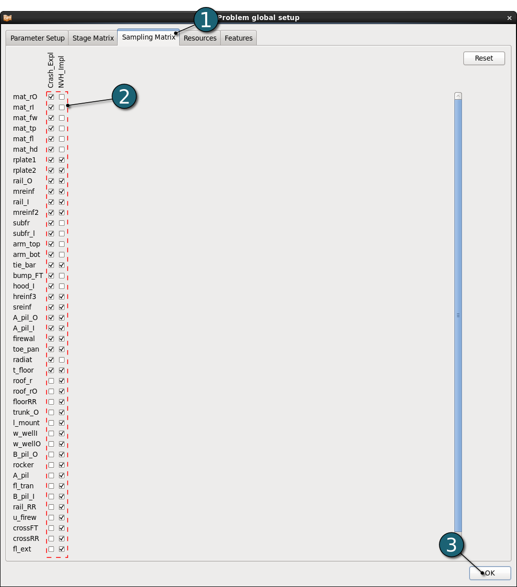
- Select the Sampling Matrix tab.
- If you don't want to use a parameter as variable for a respective sampling, the variables can be switched off here. The parameters are treated as constants then.
- Click on the OK button to proceed.
Home Screen Process Flowchart
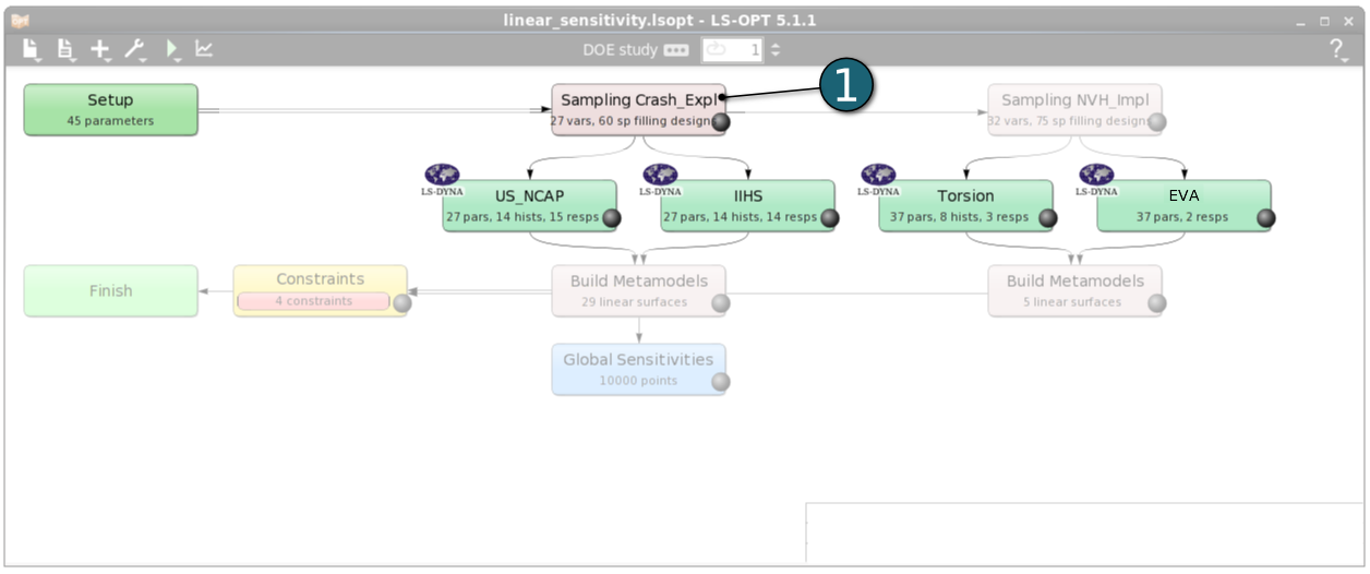
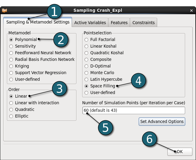
- Double click on the Sampling Crash_Expl box.
A window Sampling Crash_Expl shall open.
Define Metamodel Settings for Crash_Expl
- Select the Sampling & Metamodel Settings tab.
- For Metamodel select from the list Polynomial response surface.
- For approximation Order of the Polynomial model we take Linear.
- At this point, we took a linear polynomial metamodel, because the model is too large to be able to performe enought simulations to show nonlinearities. If possible, it's better to do more simulations and use e.g. Radial Basis Function Networks.
- Make sure that the Point Selection is set to Space Filling.
- Due to the large number of variables in this case Space Filling is chosen as Point Selection method for performance reasons.
- Type 60 for Number of Simulation Points.
(approx. 2*number of variables recommended for DOE) - Click on the OK button to proceed.
Define Metamodel Settings for NVH_Impl
- In order define the sampling NVH_Impl double click on the Sampling NVH_Impl on the Main Home Screen Process Flowchart.
- Then follow the steps 1-6 of Define Metamodel Settings for Crash_Expl above only by changing the Number of Simulation Points (step 5) to 75 because 32 variables are considered instead of 27.
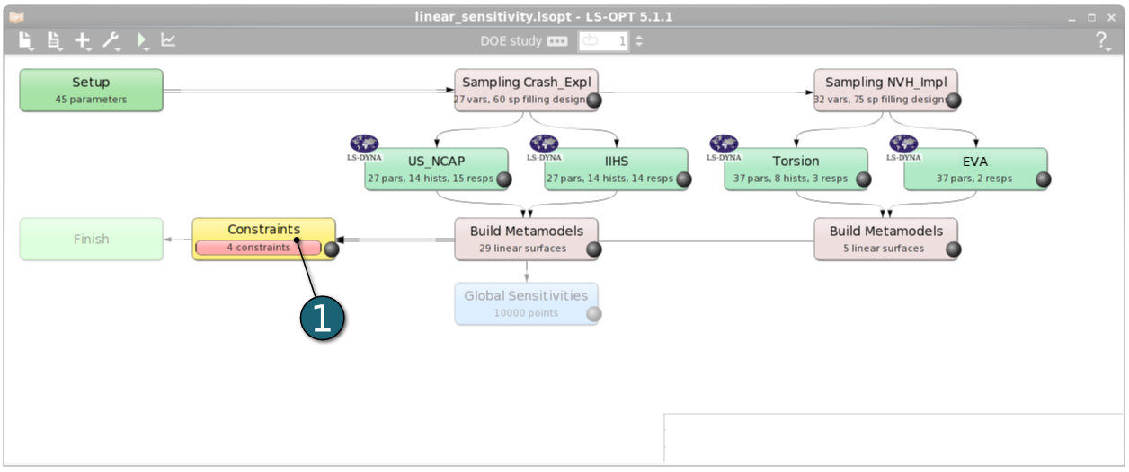
Home Screen Process Flowchart
- Double click on the Constraints box to define contraints.
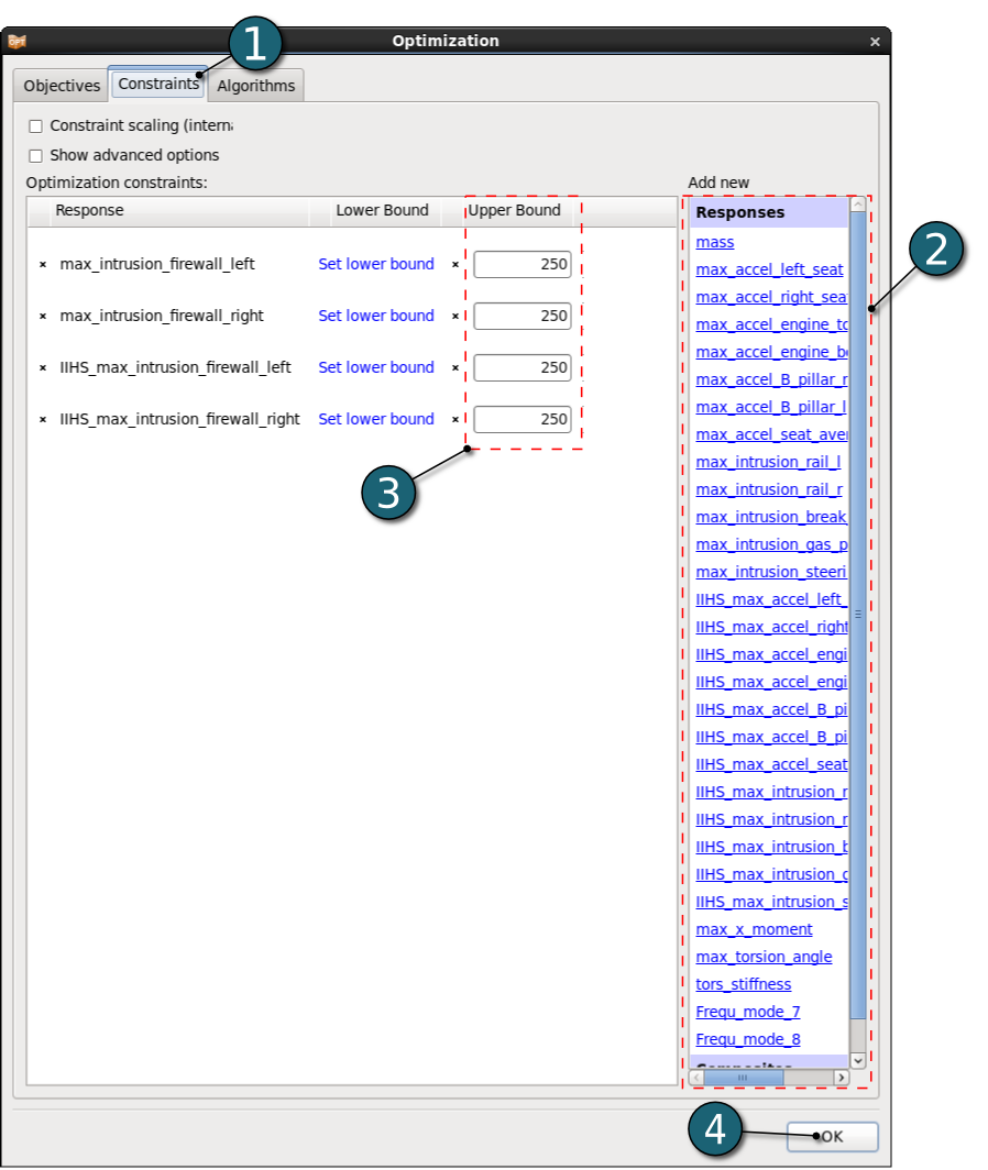
A window Optimization shall open.
Define Constraints
- Select the Constraints tab.
- Under Responses select max_intrusion_firewall_left, max_intrusion_firewall_right, IIHS_max_intrusion_firewall_left and IIHS_max_intrusion_firewall_right as constraints.
- Select Set upper bound and enter 250.
- Click on the OK button to proceed.
Home Screen Process Flowchart
Run LS-OPT
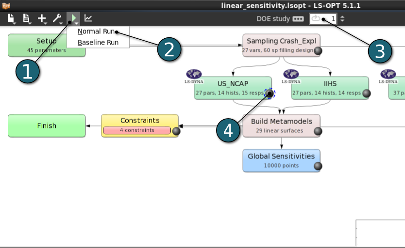
- Click on the Run button on the Control Bar.
- Click on the Normal Run.
- The user can get information on the status of the current iteration during execution.
- For every stage the user has the option to observe the progress of the program execution by selecting the LED at the corner on the Stage box. It is possible to observe the Progress and View Log for more information about the execution process.
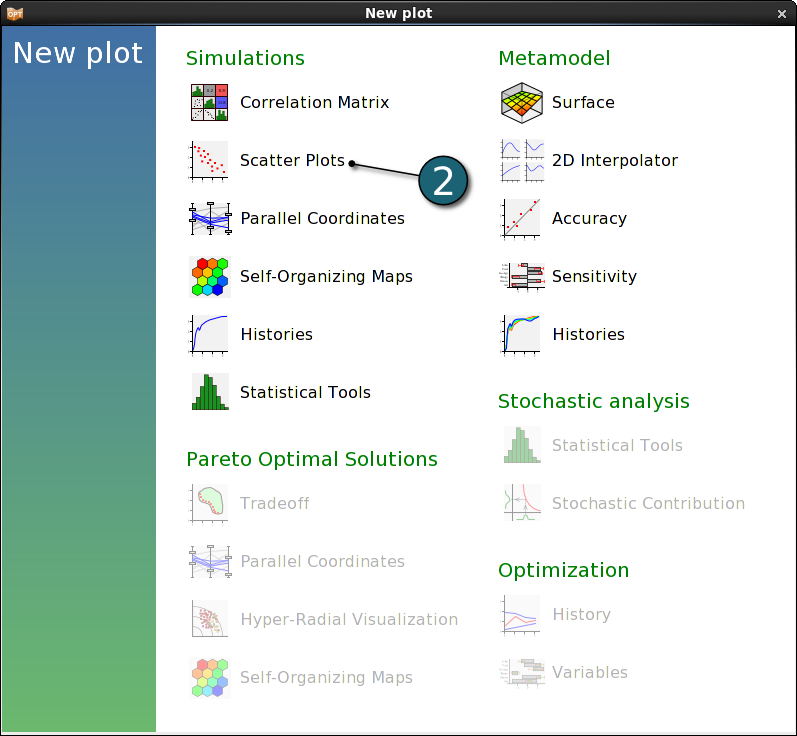
Results of the simulated points for the selected iterations appear as dots on the scatter plots. This feature allows the three-dimensional plotting of any three entities. A forth dimension may be visualised using the color of the points. 2D plots can be obtained by selecting No entity for the z axis.
Home Screen Process Flowchart
- Click on the Open the viewer button on the control bar on the Home Screen Process Flowchart.
Scatter Plot
- Choose Scatter Plots as the type of plot under Simulations.
![]()
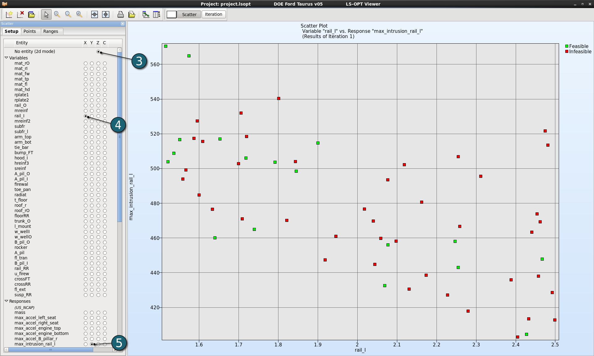
Variable "rail_l" vs. Response "max_intrusion_rail_l":
- For the Z-axis select No entity to switch to the 2d mode.
- For the X-axis select the Variable rail_l.
- For the Y-axis select the Response max_intrusion_rail_l.
Feasible points are shown in green, infeasible points in red.
The Figure shows the correlation between a variable and a response.
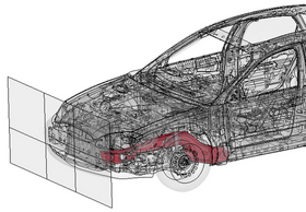
We could conclude: the bigger the thickness of the variable rail_l (see highlighted in red in the figure below), the smaller is the maximal intrusion of the response max_intrusion_rail_l.
The remaining dimensions, that could also have influence on the response, are projected into the plot.
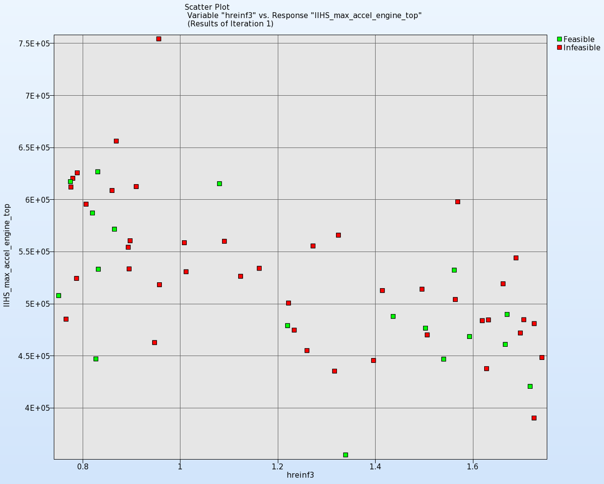
Variable "hreinf3" vs. Response "IIHS_max_accel_engine_top":
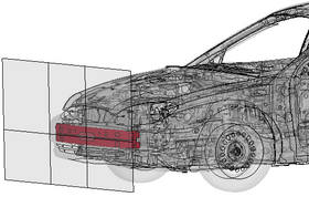
For the X-axis select the Variable hreinf3 and for Y-axis select IIHS_max_accel_engine_top.
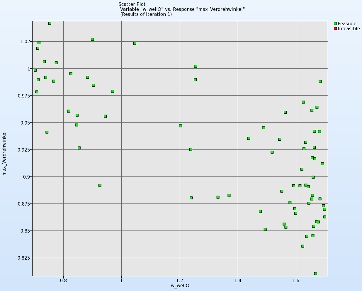
Variable "w_wellO" vs. Response "max_torsion_angle":
For the X-axis select the Variable w_wellO and for Y-axis select max_torsion_angle.
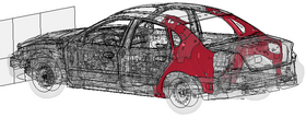
Obviously we can say: the bigger the thickness of the variable w_wellO (see highlighted in red in the figure below), the smaller is the maximal torsion angle.
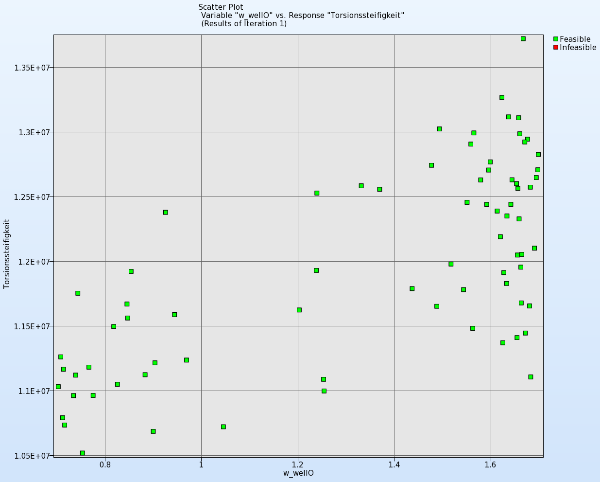
Variable "w_wellO" vs. Response "torsional_stiffness":
For the X-axis select the Variable w_wellO and for Y-axis select tors_stiffness.
We defined torsional stiffness as x-moment / torsion angle. As expected the scatter plot shows: the thicker the w_wellO, the smaller the maximal torsion angle (scatter plot above), the greater is the torsional stiffness.
This plot visualizes history curves based on time data or crossplots obtained from simulations.
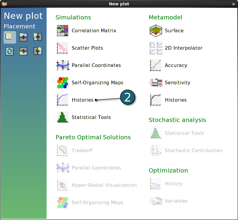
New Plot - Histories
- Click on the New Plot button on the menu bar - ( or click on the View button on the Home Screen Process Flowchart as done in previous step ).
- Select under Simulations the item Histories.

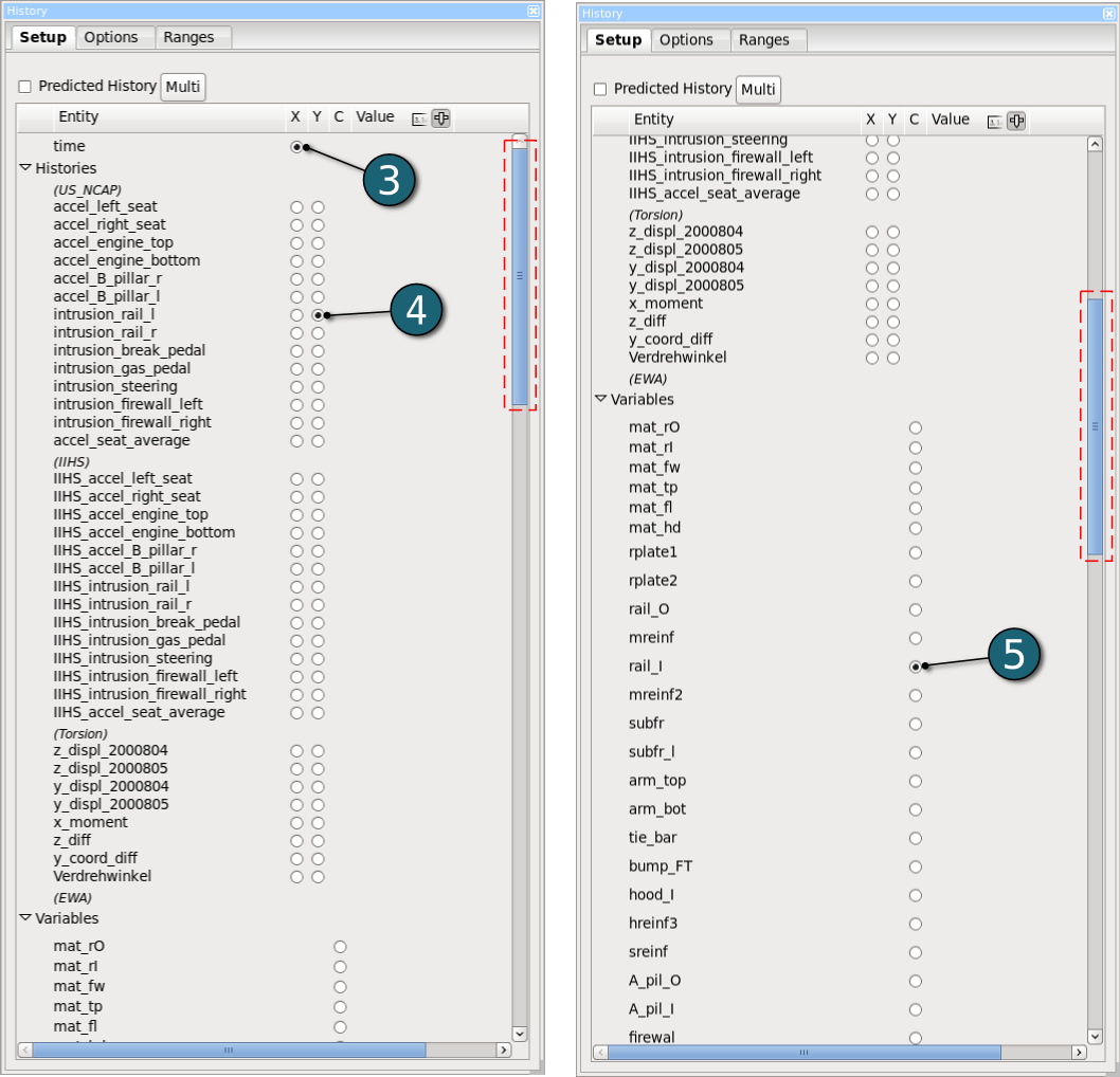
Plot History - Settings
- As x-coordinate select time.
- Choose intrusion_rail_l as y-coordinate.
- Set the variables rail_l as c-coordinate.
(C-coordinate affects the color of each curve dependend on the value of the c-coordinate.)
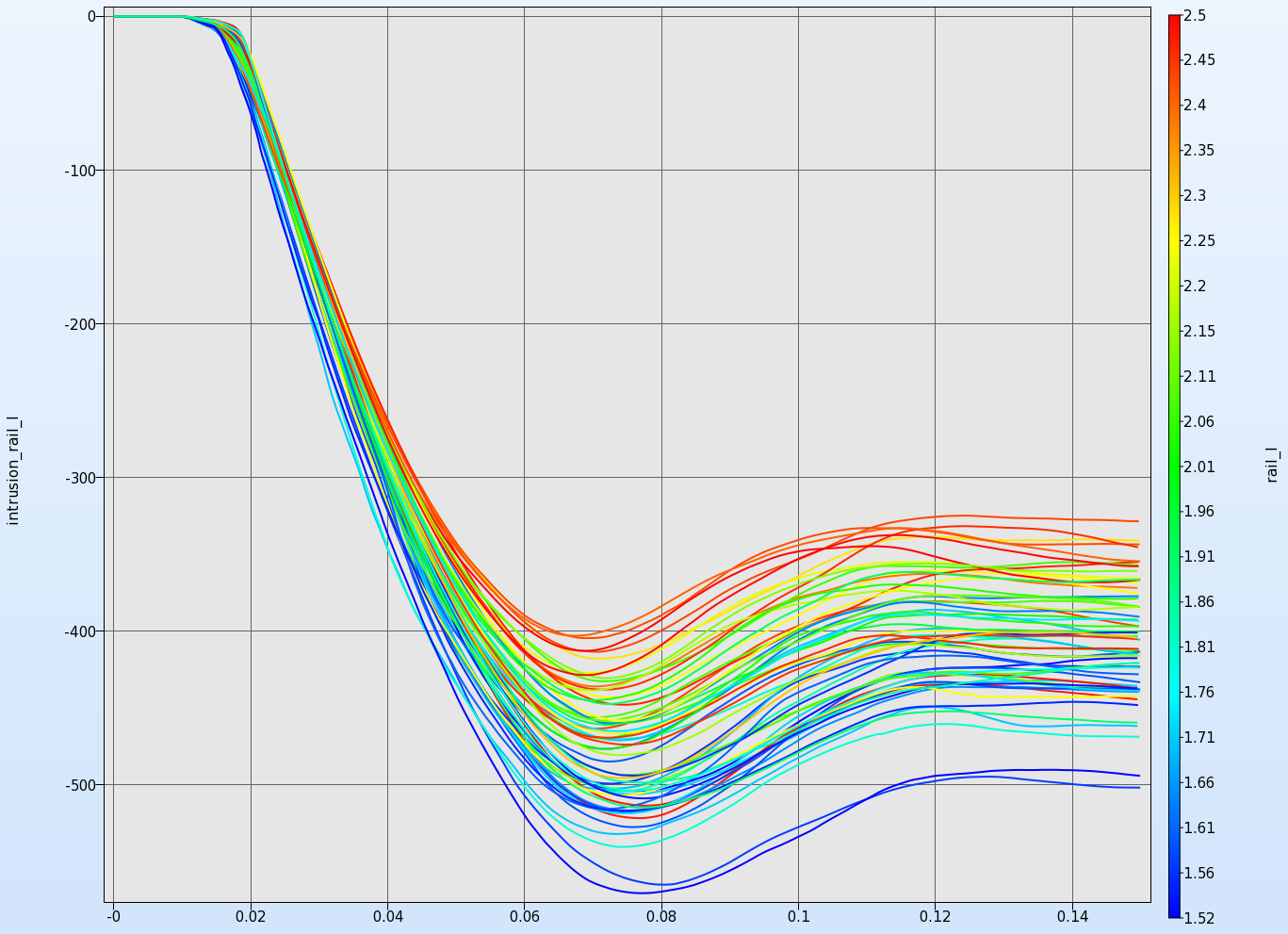
→ History curves of 60 simulations for intrusion_rail_l. The value of the variable rail_l determines the color of each curve.
There you can see, that the variable rail_l has a considerable influence on the response max_intrusion_rail_l.
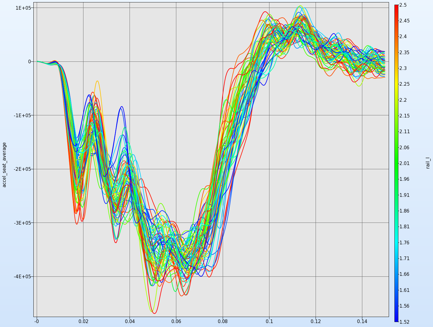
Choose now accel_seat_average as y-coordinate and leave the variable rail_l as c-coordinate.
→The chaotic behaviour does not mean inevitable, that the variable does not have an influence on the response. It could be, that the influence of other variables leads to this behaviour.
Two- or three-dimensional cross-sections of the metamodel surfaces and simulation points can be plotted and viewed from arbitrary angles.
New Plot - Surface
- Click on the New Plot button on the menu bar - ( or click on the View button on the Home Screen Process Flowchart as done in previous step for Scatter Plots).
- Select under Metamodel the item Surface.

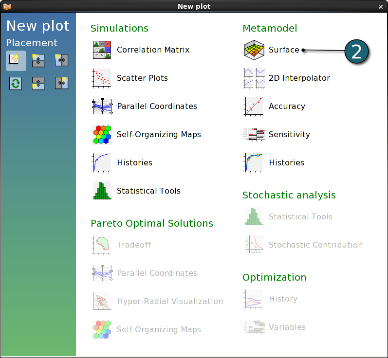
Plot Surface - Settings
- Select the Setup panel.
- Choose max_intrusion_rail_l as z-coordinate.
- Set the variables rail_l and arm_top as x- and y-coordinate, respectively.
(The sliders allow changing the variable values for unselected variables (variables not plotted). The slider for the active variables can be activated by selecting the “Predicted Value” option, a purple cross is displayed on the metamodel showing the values for the selection.) - Select Constraints.
(Constraints are displayed on the surface.
Feasible regions are in green, the shade of red shows the degree of infeasibility (number of violated constraints), the colored
line show the location where the constraints are exactly met.) - Go to the Points panel.
- Turn Iterations to All.
- Show all the feasible and infeasible points.
- Select Show Residuals.
(Shows the deviation between the metamodel and predicted values as black vertical line.)
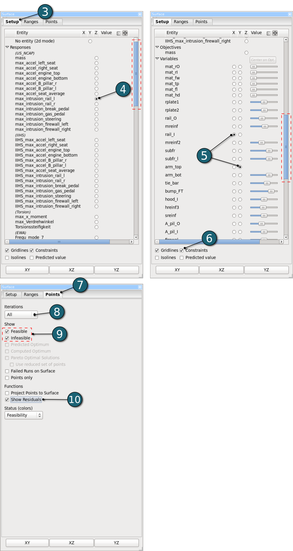
→The residuals are mainly small, thus you can say this is a well approximated metamodel.
Note the legend describing violated constraints on the top right.
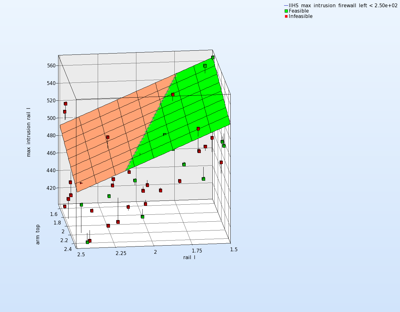
Select now for response max_intrusion_steering and for variables rail_l and A_pil_l.
→In comparison with the figure above the metamodel is not so well approximated. Almost all residuals are large.
Which variable appears to be the most important?
The significance of a variable for a response can be illustrated with ANOVA (analysis of variance) or GSA/Sobol (global sensitivity ananlysis). Note that also GSA/Sobol illutstrates only the linear influence here, because we use a linear metamodel.
New Plot - Sensitivity
- Click on the New Plot button on the menu bar - ( or click on the View button on the Home Screen Process Flowchart as done in previous step for Scatter Plots).
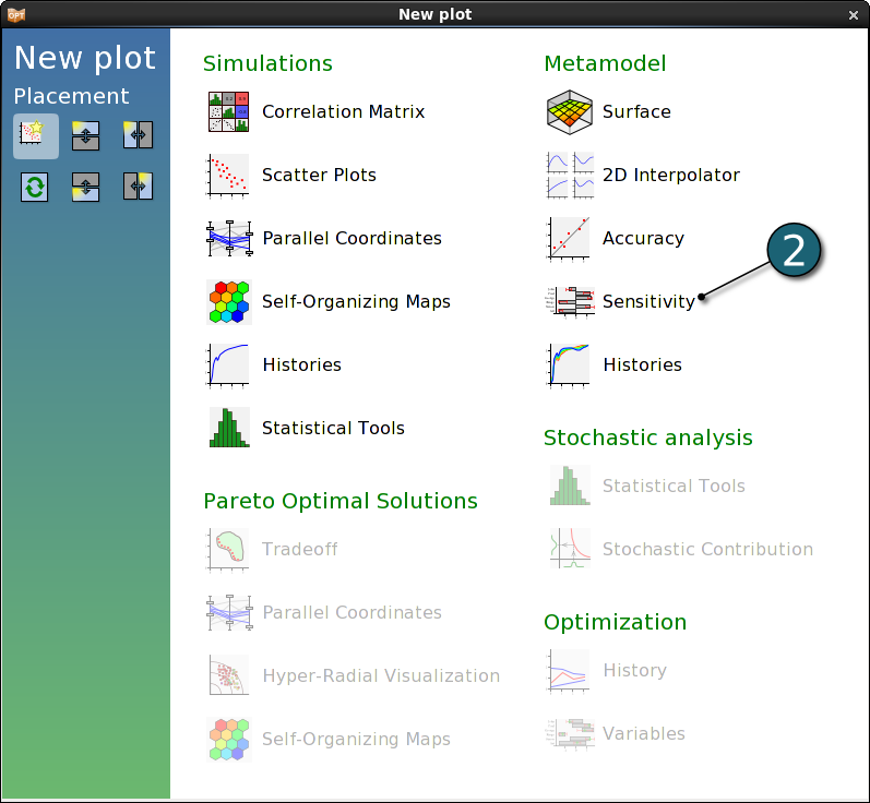
- Select under Metamodel the item Sensitivity.

ANOVA
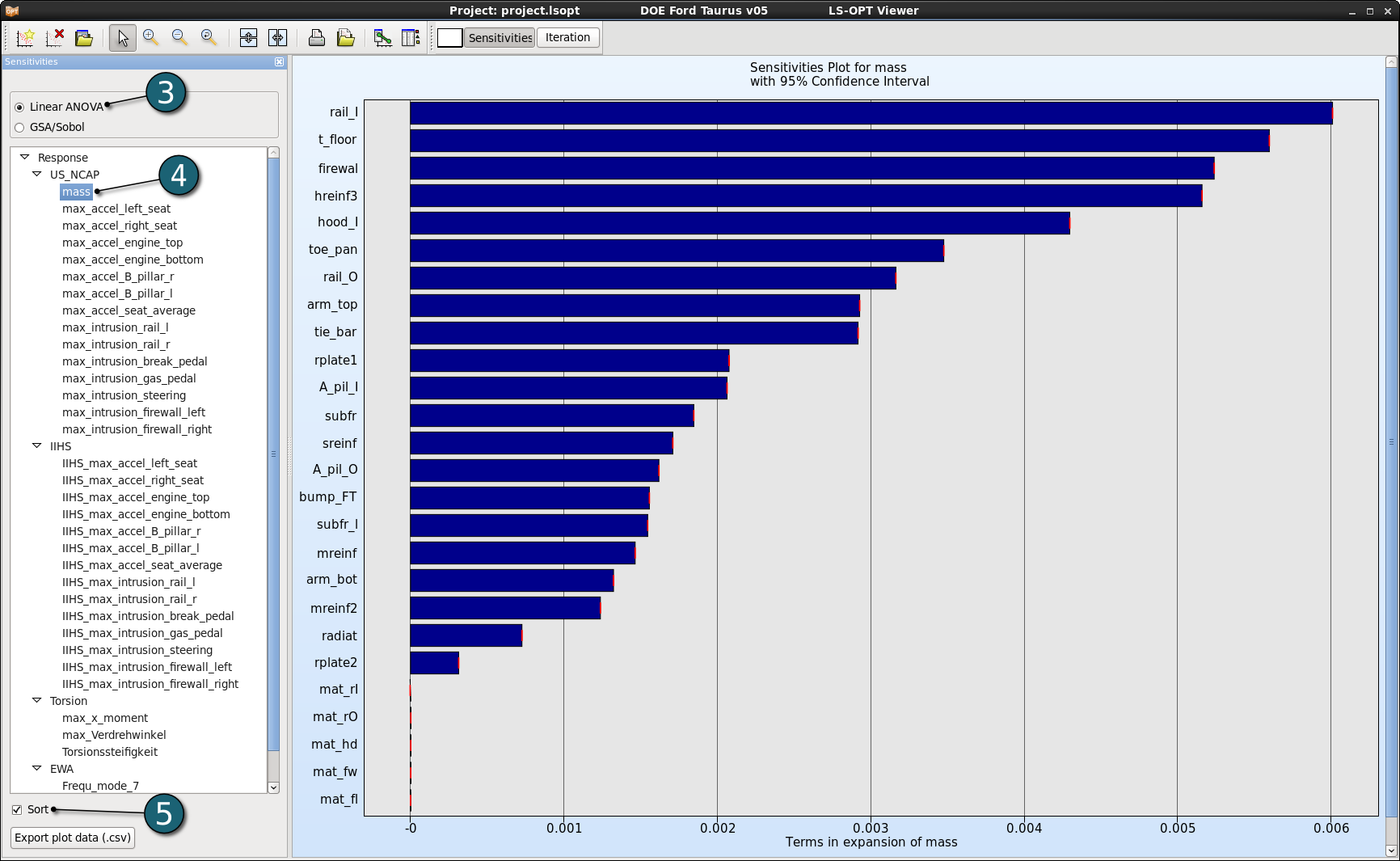
- Select Linear ANOVA in the new window.
- From Response, e.g. for the load case US_NCAP, select mass.
(The influence of different variables on response mass is shown in the Figure below.) - Sort the variables according to their significance for mass.
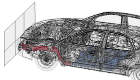
→ For the response mass the variables rail_l and t_floor are the most important variables. (They are highlighted in red and blue in the figure below .)
In contrast the variables mat_rl and mat_rO are insignificant.
The influence of different variables on response max_intrusion_rail_l:
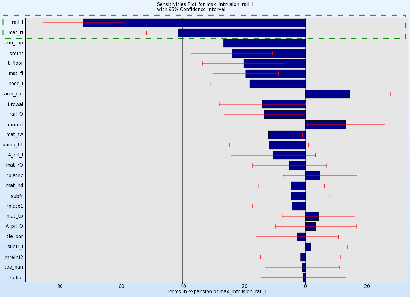
From Response select max_intrusion_rail_l for the load case US_NCAP, to see therefor the belonging diagramm.
→ rail_l and mat_rl are the most important variables.
GSA/Sobol
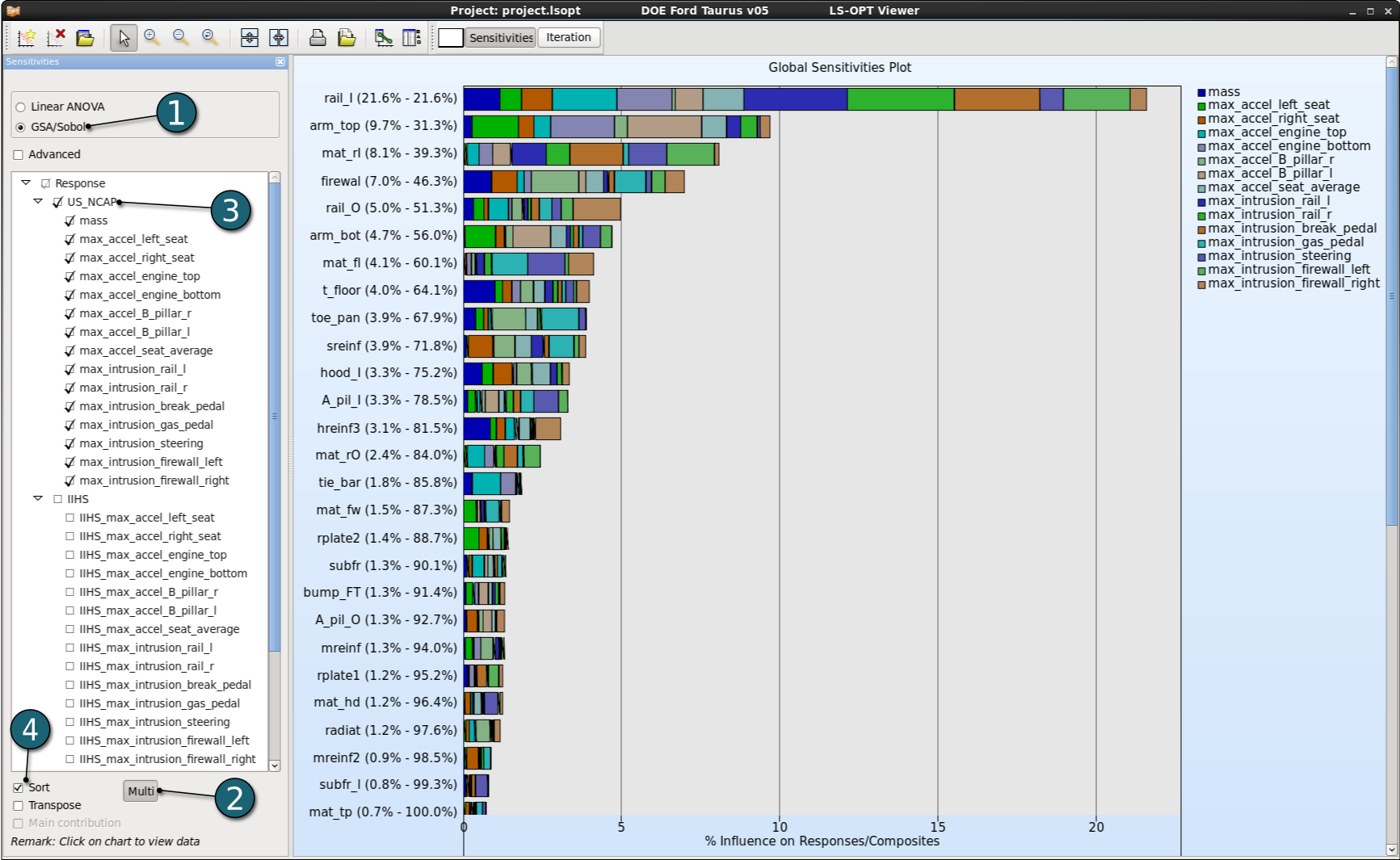
- Select the GSA/Sobol.
- Select Multi. (This option allows to select multiple responses.)
- From Response select US_NCAP.
(The influence of different variables on case US_NCAP is shown in the Figure.) - Sort the variables according to their significance for US_NCAP.
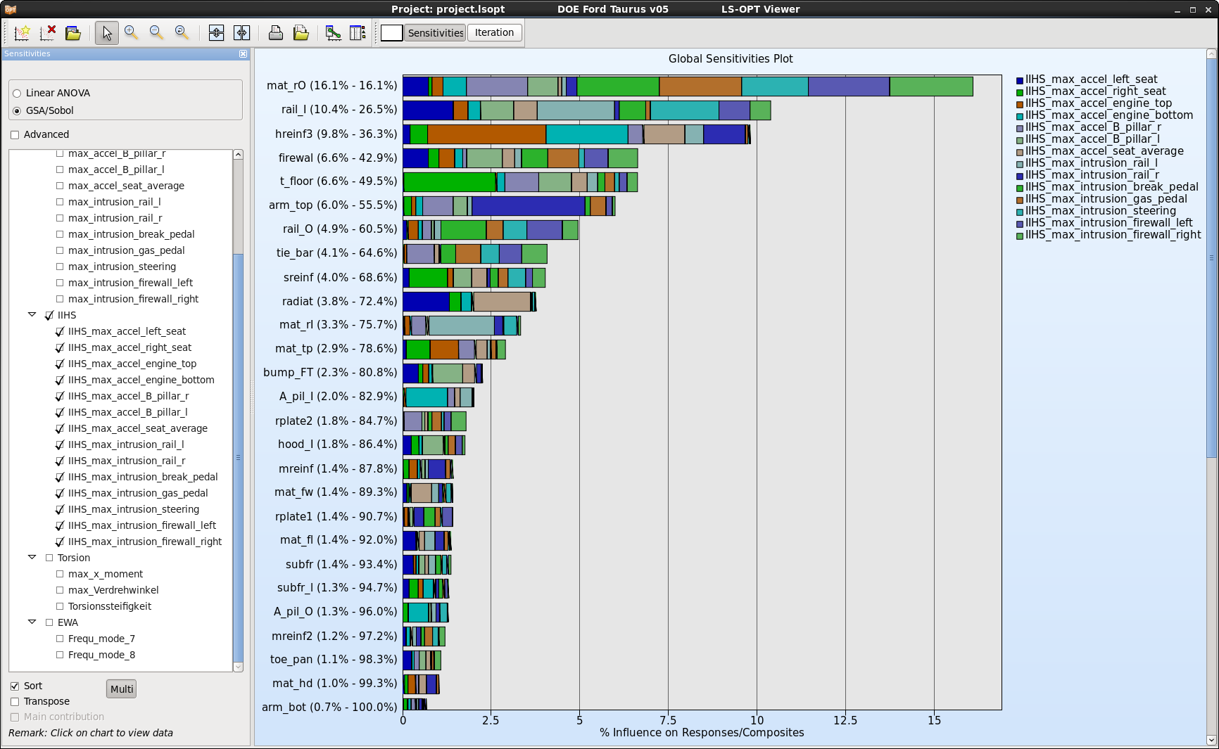
Select now from Response IIHS to see the influence of variables on this load case.
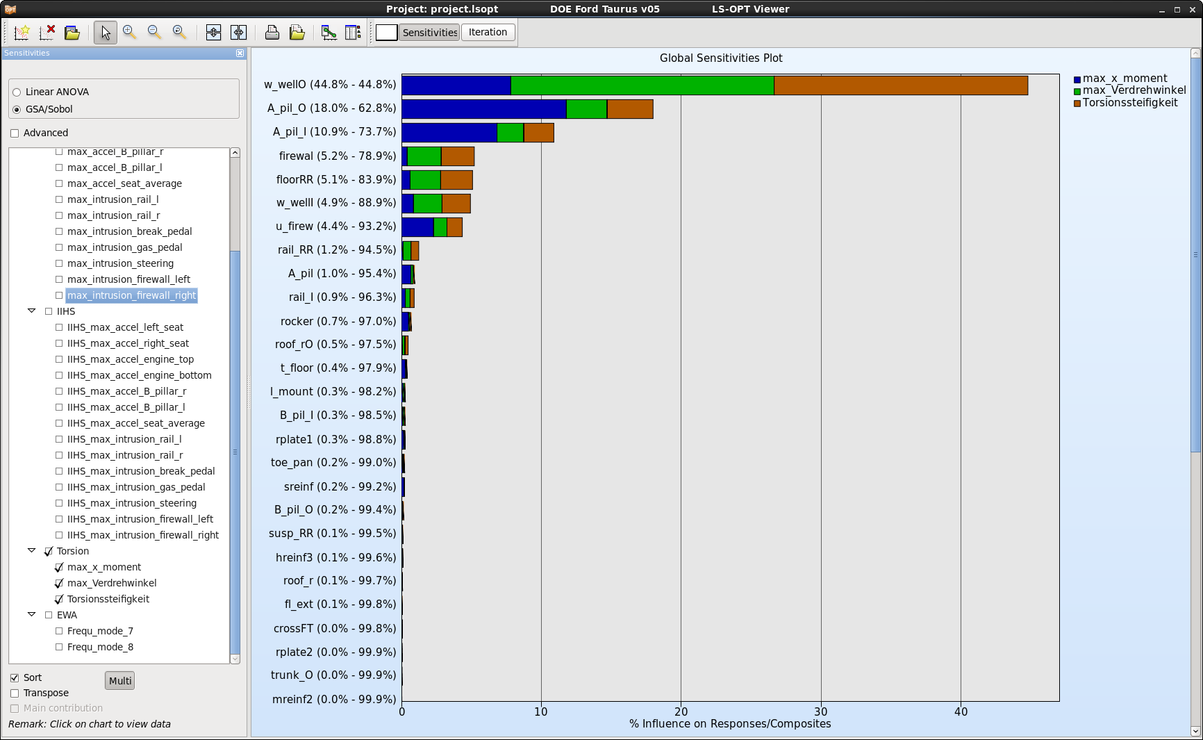
Sobol - Diagram for load case Torsion:
Sobol - Diagram for load case EVA:
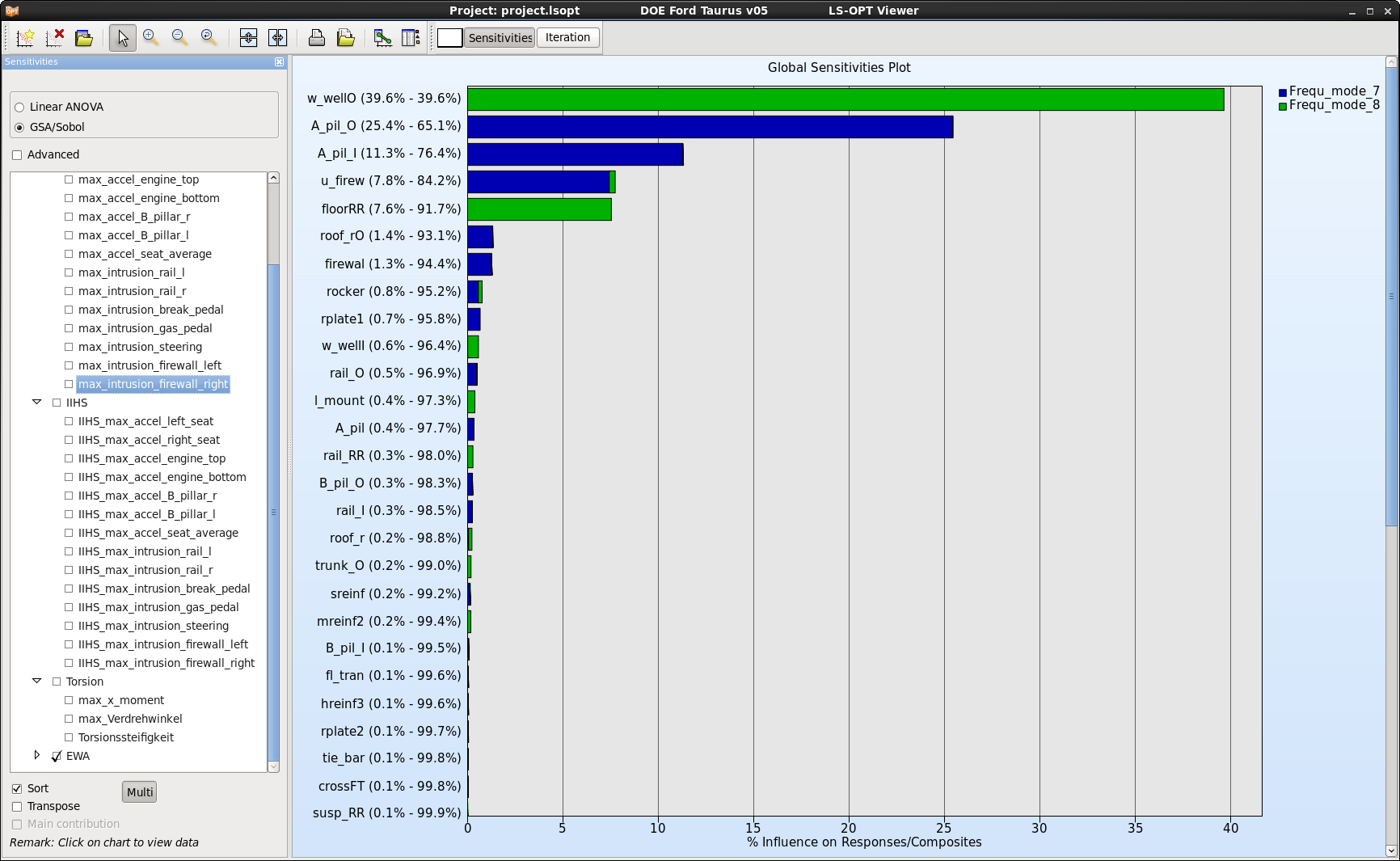
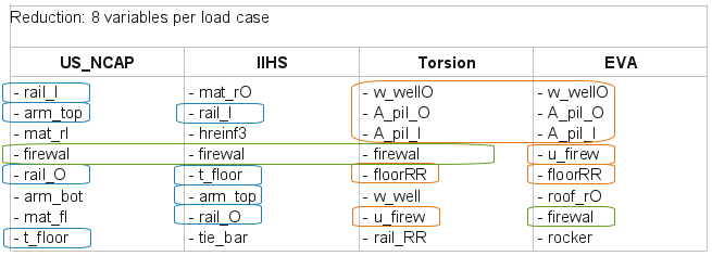
This information may be used to reduce the set of variables for each load case and e.g. perform an optimization afterwards. Here, 8 most important variables are selected for each load case. The colors in the table below visualize the common variables of the load cases. Obviously the variable firewal is important for all four load cases.
The command file is available for download:
| LS-OPT project file (.lsopt ): | linear_sensitivity |
| Input files: | US_NCAP |
| IIHS | |
| Torsion | |
| EVA |

